1. Introduction

1.1. Background

Evidence of the links between monetary policy and the price level has been the subject of much economic debate to this day. This policy is implemented by a state (the government more precisely) through any banks whose main goal is to control the money supply and ensure price stability. The development of this monetary policy is, therefore, the primary objective of any government in order to ensure the social well-being of its population.

In setting up its monetary policy, banks act on the monetary base as an operational objective, with the aim of creating a stable linear relationship between the monetary base and the money supply M2, and on the other hand between the money supply M2 and the general price level. We understand that the M2 money supply, therefore, constitutes the main objective of monetary policy which makes it possible to achieve the final objective of price stability. To act on intermediate objective M2, the Central Bank of Congo sets, as part of the economic and financial program, the quantitative objective of the monetary base. The objective of monetary policy under which the Central Bank of Congo is at the head is to achieve and maintain price stability by adjusting the supply and demand for money. To do this, the Central Bank of Congo determines the control framework through which monetary policy will be implemented during the year. From this framework, he decides to what extent to reserve or relax monetary conditions.

1.2. Problematic

Within the framework of general economic policy, monetary policy has its own points of action to achieve the main objectives of overall economic policy. It aims to act globally on real variables of the economy through monetary variables such as money supply and demand, exchange rate, interest rate.

Thus, the real role of monetary policy is to provide the sector with the quantity of money necessary for the expansion of economic activities without generating inflationary or deflationary slippage.

However, in the context of the Democratic Republic of Congo, research on welfare through monetary policy is problematic given, on the one hand, the objectives officially assigned to monetary policy, to ensure the financing of the economic development of the country and promote domestic price stability and maintenance of the external balance of payments.

Indeed, the results of monetary policy in terms of inflation rate testify to the ineffectiveness of the transmission mechanisms of monetary policy on the real variables of the Congolese economy, namely price stability.

This work, therefore, aims to assess the effect of this monetary policy on the general price level in Democratic Republic of Congo from 2000 to 2016.

1.3. Research Question

The research of our work is based around a question which is the following:

What is the impact of monetary policy on the general price level in the Democratic Republic of the Congo?

It is to this concern that we will try to answer in our methodology section which will be done a little down in our work.

1.4. Objective of the Study

The objective of our research work is to analyze and address the relationship between money supply and prices to:

- Analyze the evolution of the money supply and the prices

- Determine the impact of the money supply on prices

1.5. Hypothesis Research

- Monetary policy acts inefficiently on the general price level or even the negative impact of monetary policy on the price level resulting from the mismanagement of currency management instruments

2. Literature Review

In this part of the study, we will first do a little theoretical summary of the literature review on monetary policy, then we will empirically talk about the authors who have carried out similar work on the effect of monetary policy on awards as well as the results obtained in the Central Bank of West African States and in summary the contribution of our work dealing with the issue as well as the results that were obtained. The review focuses on the methodology for evaluating the impact of monetary policy on the various inflation variables (prices).

2.1. Theoretical Review

In this theoretical economic review of the impact of monetary policy on prices we first have the variation in the quantity of the money supply where the policy of central banks varies according to the effects attributed to variations in the money supply: effect on the price or effect on transactions, i.e. the real sphere of the economy.

Then we have the monetarist interpretation here, for monetarist economists, an increase in the money supply M causes an increase in the general price level but, does not modify the real sphere. For example, a massive rise in income leads to a general rise in prices.

Then the Keynesian interpretation which does not deny a possible (but limited) rise in prices, the increase in the money supply has above all the effect of allowing a revival in the event of sluggish growth or even recession (fall in national production).

The excess of distributed currency allows:

- An increase in income which favors the purchase of consumer goods (Keynesian multiplier principle),

- An incentive for companies to invest, with economic activity picking up again (Keynesian accelerator principle).

Economists of this tendency advocate greater credit facilities (lower interest rate) and increases in income.

And finally, the choice of monetary policies or everything, therefore, depends on the causal link admitted in the equation Mv = PT.

If we consider that a change in M causes above all a rise in prices by leaving activity unchanged, the monetary policy of central banks must be strict: control of credit, high-interest rate.

If we consider, conversely, that a little inflation is not serious if it is controlled, monetary policy will consist of lowering the key interest rate and facilitating the granting of credit by the banks. The decision to facilitate or restrict the issuance of money ultimately lies with the central bank or the system of central banks.

2.2. Empirical Review

Price stability is at the heart of most central bank objectives (ECB, 2012). Therefore, the impact of exogenous shocks on monetary policy can be assessed through its effects on price stability. Empirical studies of several research works have been carried out within the Central Bank of West African States (BCEAO) since 1996, with the aim of providing an overview of the implementation of monetary policy. This empirical work has made it possible to identify the determining factors of price dynamic within the Union.

These are: imported inflation (Dembo Toé, 2010), the analysis of the contribution of monetary policy has economic growth (Blot Christophe & Hubert Paul, 2018), the nominal effective exchange rate (Dembo Toé, 2010), the sensitivity of economic activity to monetary and budgetary shocks in Senegal (Ndiaye Cheikh T, 2016). There is also work on the analysis of the impact of monetary shocks on activity and inflation (Rafiq and Mallick, 2008; Dimitrijevic and Lovre, 2013; Mishkin, 2009; Reynard, 2007; Bonga-Bonga and Kabundi, 2015; Bikai and Kenkouo 2015; Ngerebo, 2016). B. Ngoma and B. Et-onomo (2019), Analysis of the Monetary Multiplier in the CEMAC Zone; Boketsu, J., and Diwambuena, J (2019), “Fiscal Policy And Macroeconomic Performance; Bikai, J., and Essiane, D., (2018), Monetary Policy, Monetary Stability and Economic Growth. Most of these studies used relatively similar methodologies. Overall, they constructed and estimated econometric models of the auto-regressive vector (VAR) or error correction models (ECM). This model includes explanatory variables, the money supply (M2) and the interest rate for tenders on the money market.

NDIAYE LEO (2016) analyzed the sensitivity of economic activity in Senegal to structural VAR shocks in monetary and fiscal policies. The results of the estimates that emerge there show that monetary policy fulfills its objective of stabilizing prices and remains neutral against economic activity in Senegal with a short delay in transmitting shocks. It also reveals that monetary policy reacts to shocks affecting fiscal policy in Senegal and the results of the Granger causality analysis reveal the exogenous nature of the monetary and the fiscal policy.

BLOT Christophe and HUBERT Paul (2018) evaluated the contribution of monetary policy to economic activity in the Euro zone, the United States and the United Kingdom from 1990 to 2018. Their analysis indicates that monetary policy has an effect significant on GDP in these six countries, with fairly long transmission times. This amounts to saying that the currency is not neutral there, because it impact in the real sector in these six economies.

In developing countries, some authors highlight the weakness of the transmission channels for monetary policy and particularly the interest rate channel, due to the weakness of the institutional framework, embryonic financial markets, banking excess liquidity, the persistence of fiduciary circulation, the weakness and instability of monetary and credit multipliers as well as the preponderance of the banking sector (Mishra and al. 2013; Mishra and al. 2016; Matata, 2019). Other authors, on the other hand, conclude with the efficiency of transmission channels in some developing countries (Saad, Mohammed and Zakaria, 2011; Berg and al 2013). However, there seems to be a consensus that the interest rate channel is more efficient in countries with sufficiently developed financial markets (Mishra and al., 2013, 2016; Davoodi and al., 2013). The work of Davoodi and al. (2013) show that the use of standard statistical inferences always results in weak transmission mechanisms in developing countries.

In sub-Saharan Africa, several studies have addressed this theme, most of which confirm the weakness of the interest rate channel in the CAEMC (Central Africa Economic and Monetary Community) region (Kamgna and Ndambendia, 2008; Bikaiet Kenkouo, 2015). In other words, changes in the key rate of the Bank of Central African States have little or no effect on activity and prices. None of these studies, however, looked at the impact of the interest rate on external monetary stability and mainly on foreign exchange reserve.

Other empirical studies conducted in other countries in sub-Saharan Africa have shown the impact of currency and the output gap on inflation. Barnichon and Peiris (IMF, 2008) used as an explanatory variable for inflation in sub-Saharan African countries: the output gap, currency (real currency gap: the difference between money supply and demand) and precipitation. The results of their study give elasticities of 0.28 for the output gap, 0.34 for money and -0.13 for precipitation. The elasticity of the output gap is 0.42 for countries outside the CFA zone and 0.32 for the countries of the CFA zone in the sample (Cameroon, Ivory Coast, Mali, Niger, and Senegal). The elasticity of the currency is also higher in countries outside the CFA zone (0.37) than in countries in the CFA zone (0.15). Ocran (2007), in an inflation model for Ghana, obtains an elasticity of the money supply of 0.42. On the other hand, Kovanen (IMF, 2011), shows that the currency explains little the evolution of prices in Ghana and obtains an elasticity of the output gap with respect to inflation of 0.91. Several studies also indicate the role of the inertia of inflation in most countries of sub-Saharan Africa and the weak capacity to explain the evolution of inflation by those of money. For the UEMOA zone, Dembo Toé and Hounkpatin (2007) show that the current level of inflation depends strongly on the past value of price variations. Thus, the forecast error of the IHPC in UEMOA is due to 82.6% to its own innovations, 3.8% to those of the nominal effective exchange rate, and 8.8% to the evolution of import inflation and 4.8% to changes in the money supply.

2.3. Summary of the Empirical Review

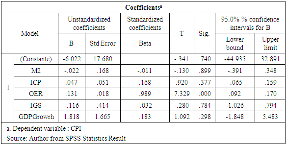
After having empirically reviewed and enumerated in the context of monetary policy what all the authors did and obtained as results in their research, it emerges in summary from our study based on the impact of monetary policy on the level general prices in the Democratic Republic of Congo (DR Congo), that the currency explains little the evolution of prices. Evaluating the test at an alpha of 0.5 clearly showed us that: M2 has a negative amount of -0.022 but it is not significant on the CPI because its p-value = 0.899 is greater than 0.5. In this case, M2 does not have a great influence on the CPI which means that the monetary policy of the central bank of Congo (CBC) has not reached its objective of price stabilization, i.e. 95.6% of the rise in the general price level is explained by the poor monetary policy of the Congo's central bank during the period 2000 to 2016. This also matches and confirms certain empirical works listed such as that of Kovanen (IMF, 2011), which also shows that the currency explains little the evolution of prices in Ghana and obtains an elasticity of the output gap with respect to inflation of 0.91.

3. Methodology

In this work, we propose to study the effect of monetary policy on prices in the Democratic Republic of Congo. And like any scientific work, we will try to shed light on our study through the data collected at the level of the World Bank starting from 2000 to 2016 and make the regression through the use of the SPSS software. This will allow us to see through the results that we are going to obtain whether the money supply influences prices or the reverse. So, for our study, we will test empirically, using series econometrics techniques.

3.1. Presentation of the Variables and the Model

For our study, we propose the following variables based on the data available from 2000 to 2016 to explain the impact of monetary policy on prices in the Democratic Republic of Congo. We will therefore show the relationship between money supply and prices. In order to show this relationship, our model will be made up of the following variables: Consumer Price Index (CPI), money supply (M2), GDP growth (annual%), Imports of goods and services (IGS), Official exchange rate (OER), Inflation, consumer prices (ICP).

Based on the variables mentioned, our model can take the following form:

With the constant and : the error term Coefficient of independent variables

CPI = Consumer Price Index

M2 = Money supply

ICP = Inflation consumer price

OER = Official exchange rate

GDPgrowth = Gross domestic product

IGS = Imports goods and services

3.2. Definition of Variables

v Consumer Price Index (2010 = 100)

Consumer price index reflects changes in the cost to the average consumer of acquiring a basket of goods and services that may be fixed or changed at specified intervals, such as yearly. Consumer price indexes are constructed explicitly, using surveys of the cost of a defined basket of consumer goods and services.

A general and continuing increase in an economy’s price level is called inflation. The increase in the average prices of goods and services in the economy should be distinguished from a change in the relative prices of individual goods and services. Generally accompanying an overall increase in the price level is a change in the structure of relative prices, but it is only the average increase, not the relative price changes, that constitutes inflation. A commonly used measure of inflation is the consumer price index, which measures the prices of a representative basket of goods and services purchased by a typical household. The consumer price index is usually calculated on the basis of periodic surveys of consumer prices. Other price indices are derived implicitly from indexes of current and constant price series.

v GDP growth (annual %)

Gross domestic product (GDP) represents the sum of value added by all its producers. Value added is the value of the gross output of producers less the value of intermediate goods and services consumed in production, before accounting for consumption of fixed capital in production. The United Nations System of National Accounts calls for value added to be valued at either basic prices (excluding net taxes on products) or producer prices (including net taxes on products paid by producers but excluding sales or value added taxes). Both valuations exclude transport charges that are invoiced separately by producers. Total GDP is measured at purchaser prices. Value added by industry is normally measured at basic prices. When value added is measured at producer prices. Growth rates of GDP and its components are calculated using the least squares method and constant price data in the local currency. Constant price U.S. dollar series are used to calculate regional and income group growth rates. Local currency series are converted to constant U.S. dollars using an exchange rate in the common reference year.

v Imports of goods and services (% of GDP)

Imports of goods and services represent the value of all goods and other market services received from the rest of the world. They include the value of merchandise, freight, insurance, transport, travel, royalties, license fees, and other services, such as communication, construction, financial, information, business, personal, and government services. They exclude compensation of employees and investment income (formerly called factor services) and transfer payments.

v Money supply M2

Money and the financial accounts that record the supply of money lie at the heart of a country’s financial system. There are several commonly used definitions of the money supply. The narrowest, M1, encompasses currency held by the public and demand deposits with banks. M2 includes M1 plus time and savings deposits with banks that require prior notice for withdrawal. M3 includes M2 as well as various money market instruments, such as certificates of deposit issued by banks, bank deposits denominated in foreign currency, and deposits with financial institutions other than banks. However defined, money is a liability of the banking system, distinguished from other bank liabilities by the special role it plays as a medium of exchange, a unit of account, and a store of value.

v Official exchange rate

Official exchange rate refers to the exchange rate determined by national authorities or to the rate determined in the legally sanctioned exchange market. It is calculated as an annual average based on monthly averages (local currency units relative to the U.S. dollar).

v Inflation, consumer prices (annual %)

Inflation as measured by the consumer price index reflects the annual percentage change in the cost to the average consumer of acquiring a basket of goods and services that may be fixed or changed at specified intervals, such as yearly.

3.3. Empirical Analysis Results of the Descriptive Approach

This section allows us to make a descriptive analysis of the different trends of each variable used in our study from the period 2000 to 2016. And finally, we will present the results of our regression and we will analyze the results obtained describing the impact of the monetary policy on the general prices level in the Democratic Republic of the Congo.

The evolution of the broad money supply increased by 13.4% between the end of 2015 and the end of October 2016, against an increase of 5.2% a year earlier. This result is the combination of a 12% increase in the foreign currency money supply expressed in national currency and a 14.3% increase in the national currency money supply. The increase in the money supply in the national currency (200 billion CDF) could be explained mainly by the change in net claims on the State from the banking sector, which increased by 192 billion CDF. The dynamics of foreign currency deposits are more difficult to explain. Indeed, the 12% increase in the currency supply expressed in national currency turns out to be a 4.5% drop when we take into account the depreciation of the Congolese Franc. This corresponds to a drop in foreign currency deposits of US $ 142 million, but it is difficult to determine whether these are transfers abroad or an increase in foreign currency liquidity held outside the banking system.

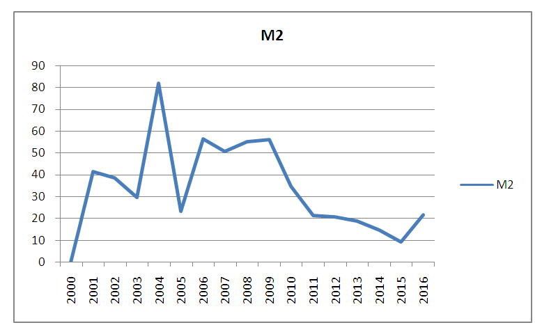Figure 1. Money supply M2 from 2000 to 2016 (Source: Author World Bank)

The general consumer price index increased by 1.3% in 2015 against 1.2% in 2014. The upward trend has been confirmed since September 2015, with an average monthly inflation rate of 1.5% for the four last months of 2015 and 3.3% for the first ten months of 2016. It was exactly in 2016 that the highest value of 133.85 was recorded and in 2000 the lowest value of 6.80. On the basis of the available data, we can estimate that in 2025 the value should oscillate around 162. This forecast presents a relatively high level of reliability since the available values have a rather linear structure, despite notable variations (correlation coefficient = 0.79 and coefficient of determination = 0.62).

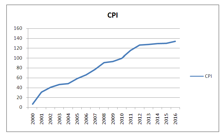Figure 2. Consumer price index (2010=100) from 2000 to 2016 (Source: Author World Bank)

The dynamics of inflation are driven by the food product price index which increased by 1.7% in 2015 against 1.5% in 2014. This index increased by 134.0% on average between the end of 2015 and 2016. Moreover, since the DRC imports refined oil, inflation should have benefited from the drop in the price of a barrel. However, the government did not lower gasoline prices at the pump until the beginning of 2015 and that in January precisely and, in proportions that do not reflect the fall in world prices, and kept stable until 2016.

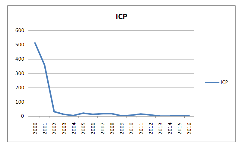Figure 3. Inflation consumer price from 2000 to 2016 (Source: Author World Bank)

For the entire period 1960-2019, there is an annual average of 257.93. It is in 2019 that we record the highest value of 1010.76 and it is in 2000 that we record the lowest value of 21.82. We can estimate from our available data that in 2025 the value should oscillate around 2761. This forecast has a relatively high level of reliability since the available values have a rather linear structure, despite notable variations (correlation coefficient = 0.78 and coefficient of determination = 0.6).

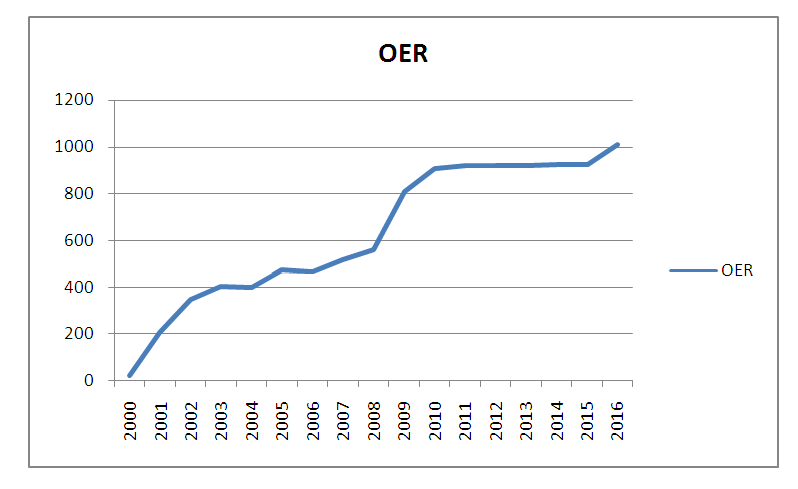Figure 4. Official exchange rate evolution from 2000 to 2016 (Source: Author World Bank)

For the period 2000-2016 as a whole, the change recorded between the first and the last year is 88%. The highest value of 49.64 was recorded in 2010 and the lowest 13.05 was recorded in 2001. Based on the available data, we can estimate that in 2025 the value should hover around 29.95. This forecast has a relatively high level of reliability since the available values have a rather linear structure, despite notable variations (correlation coefficient = 0.68 and coefficient of determination = 0.46).

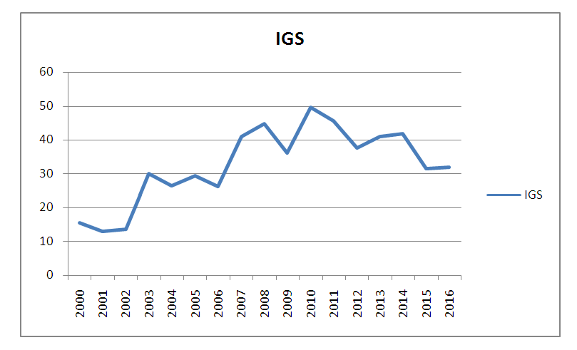Figure 5. Imports of goods and services (Source: Author World Bank)

After a strong acceleration to nearly 9% between 2013 and 2014, the GDP growth rate slowed down to 6.9% in 2015, a level markedly close to that observed in 2009 and 2010. We observe a large drop in the growth of GDP in 2016. This drop is due to a slow recovery in the extractive industries that cannot meet global demand, as well as the expansion of agriculture and services. There is also the slow resumption of domestic revenue mobilization that would restore some fiscal room for maneuver and recovery in public spending. Indeed, the added value of the extractive industries increased by only 4.8%, against an initial projection of 16.7% when the GDP growth rate was projected at 10.4%. collected to make our regression that is to say from 2000 to 2016, it is in 2014 that we record the highest value of 9.47% and it is in 2000 that we record the highest value low -6.91%. And, based on the data we have, we can estimate that in 2025 the value of GDP growth should hover around -3.47.

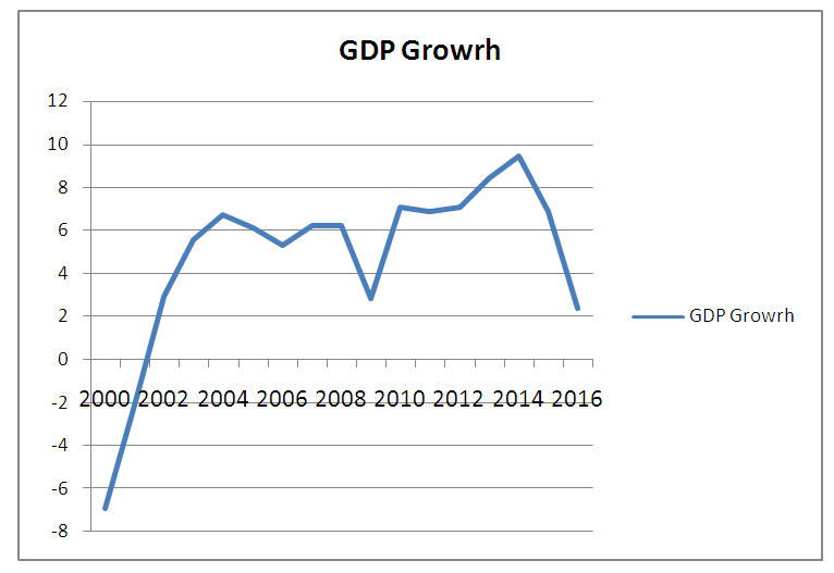Figure 6. GDPGrowth Evolution from 2000 to 2016 (Source: Author World Bank)

4. Econometric Results

We will present the tables of the results obtained during the regression of our data on the SPSS software ranging from 2000 to 2016 and interpret the results obtained.

Table 1. Observation of the variables Result

Table 2. Pearson Correlation matrix regression results from 2000 to 2016

We can indeed notice in this table 2 that all the variables mentioned and used in our formula have all been taken into account to perform linear regression on SPSS statistics software. This confirms that we have the variables M2, ICP, OER, IGS, and GDPgrowth as independent and CPI as dependent variable.

Pearson correlation measures the degree of the linear relationship between two variables. We mean by a linear relationship that the relationship can be well characterized by the straight line. Straight-line does a wonderful job of representing the relationship.

Correlation ranges always from negative 1.0 to positive 1.0 (-1.0 to +1.0). Pearson is given by a letter of PPMCC (Pearson product moment correlation coefficient) or PCC (Pearson correlation coefficient) or Pearson’s r.

For the «sig» using an alpha of 0.05 and 2-tailed tests where a two-tailed test allow for a positive correlation or a negative correlation we can use the following decision rule as we have for all of the tests

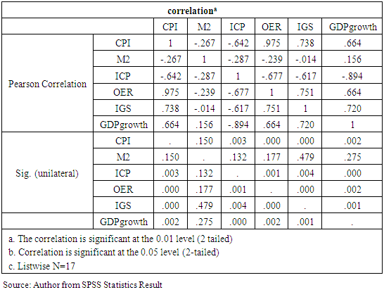
- If the p-value is less than or equal at 0.05 (p-value0.05) the test is significant that means there is a significant relationship between the dependent variable and the independent variable

- If the p-value is greater than 0.05 (p-value>0.05) the test is not significant which means there is not a relationship between the variables

So for our case here we can observe in our table 2 there are three positive correlations between CPI and OER, IGS and GDPGrowth and two negative correlations between CPI and M2 and ICP.

By continuing to argument OER and IGS are positively correlated and significant at the 0.01 level. Which means that OER and IGS contribute respectively at 9.75% and 7.38% on CPI. The GDPGrowth is positively correlated and significant at the threshold of 0.05 this implies that the GDPGrowth contributes at 6.64% in the CPI in DR Congo.

The M2 and ICP as for them they have an inverse relationship which mean the more M2 and ICP increase ICP decreases.

Let’s continue to look at the analysis of our regression tests in the next table call Durbin-Watson table in order to test the conformity of the factors that affect ICP in DR Congo.

In the table 3 title Durbin-Watson model summary result, the multiple linear regression method was used to perform the Durbin-Watson test, which consists in verifying the error independence hypothesis. What we are going to focus the most here and to explain in the table 3 is Durbin-Watson and the

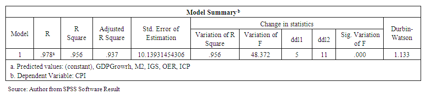Table 3. Durbin-Watson Result Model Summary

- Concerning Durbin-Watson, as we know it already in Its definition the Durbin Watson (DW) statistic is a test for autocorrelation in the residuals from a statistical regression analysis. He will always have a value between 0 and 4. A value of 2.0 means that there is no autocorrelation detected in the sample. Values from 0 to less than 2 indicate positive autocorrelation and values from 2 to 4 indicate negative autocorrelation.

Savin and White If D> DU, there is no correlation; if D< DL, there is a positive correlation; if D is between the two limits, the test is not conclusive.

Durbin, J. and Watson, G.S. (1951), Testing for serial correlation in least squares regression II, the test statistic is determined as follows: (4 - D). If (4 - D)> DU, there is no correlation; if (4 - D) <DL, there is a negative correlation; if (4 - D) is between the two limits, the test is not conclusive.

In our study, the result of Durbin-Watson value is 1.133, which indicates that the assumption that the error terms are independent has been fulfilled.

- The as for him in its definition is the measure of the amount of variance in dependent variable that the independent variables account for when taken as a group. Its measurement is not based on how much an individual predictor or a given individual variable represents, but only when we take them all as a group, this model summary table says overall, the regression model, which is what is referred to sometimes as a model, these five (5) predictors predicting CPI that overall model account for 95.6% of the variance. And as we can see in the table 3 the amount of the is 0.956 which is equal to 95.6, which simply means taken as a set the predictor M2, ICP, OER, IGS, and GDPGrowth account of 95.6% of the variance in CPI.

Table 4. Variance analysis result

The ANOVA table is the test to know if this R Squared is significantly greater than 0. It indicates the general probability of our model. In the ANOVA table, the result shows that there is a significant relationship between the five (5) predictor variables and the dependent variable at the 0.05 level of significance, where p <0.05. And if we look at our table here we find that in the column labeled ‘’Sig’’ that p-value=0.000 is less than 0.5 which means that the regression of our test is significant, is significant at 0.

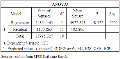
The p-value being less than 0.5 we know that the value of is significant and greater than 0 and this means that our independent variables are capable of taking into account a significant amount of variance in CPI. So in other words, the regression model is significant.

We must not forget that everything else equals any threshold is significant, when the probability, that is to say that the p value is less than 1%, we say that the model is globally significant at the threshold of 1%, when the p value is less than 5%, we say that the model is globally significant at the 5% threshold and, when the p value is less than 10%, we say that the model is globally significant at the 10% threshold.

ANOVA table (test with alpha = 0.5)

The regression model is globally significant and here we have F (5 and 11) for the regression and residual = 48.372, p<0.01, R square = 95.6.

This is to tell us that our regression analysis is statistically significant when I take these five (5) predictors together as a group, they predict CPI significantly.

Opposite to the first two summary tables of the model and ANOVA which examine the regression analysis as a whole, where the variables are taken as a whole, the table of coefficients on the other hand examines each of the predictors or variables individually. Basically we can say it is the probability of each of the variables that we used in the model to make our regression also called p-value. And what we are doing here is that we are going to look at each of our predictors and we want to zero out on it the Sig column, which are again the p-values of each of the tests. However, in this analysis, our constant has absolutely no importance. We will just focus on the five (5) p-values of M2, ICP, OER, IGS, and GDP Growth. So we will evaluate each of these tests at an alpha of 0.5 by looking at it we see that:

Table 5. Coefficient regression result analysis for the dependant variable CPI

- M2 has a negative amount of -0.022 but it is not significant on CPI because its p-value = 0.899 which is greater than 0.5 which is our alpha threshold. In this case M2 does not have big influence in CPI

- ICP has a positive amount of 0.047 and is significant on CPI with its p-value = 0.377 which mean that ICP explained a significant amount of unique variance in CPI

- OER has a positive amount of 0.131 and is significant on CPI because its p-value = 0 which is less than 0.05 we can write it like p<0.05 which mean that OER also explained a significant amount of unique variance in CPI

- IGS has a negative amount of -0.116 and is not significant on CPI because its p-value = 0.784 which is greater than 0.5 which is our alpha threshold, this simply mean IGS does not have big influence in CPI

- GDP Growth has a positive amount of 1.818 and is significant on CPI because its p-value = 0.298 which mean that GDP Growth also explained a significant amount of unique variance in CPI

5. Conclusions

Our present work aimed to assess the effect of monetary policy on the general price level in the Democratic Republic of Congo, from 2000 to 2016. After analysis and interpretation of the results via the linear regression which was carried out, we observe that our assumptions have been confirmed. our assumptions were based on the idea that the monetary policy of the central bank of the democratic republic of the Congo acts inefficiently on the general price level; the results of the calculation carried out through the SPSS software show that the monetary policy of the central bank of Congo has a negative impact on the general price level, i.e. 83% of the cover of the general price level is explained by the bad monetary policy of the Congo's central bank from 2000 to 2016.

In view of the clarifications due to the tests carried out above, it appears that the responsibility for the ineffectiveness of monetary policy in the Democratic Republic of the Congo lies both with the government and with the monetary authority which is the central bank of Congo, being given its proven inability to resist government pressure to grant advances to fill the budget deficit which is in most cases the source of the generalized price cover, ie inflation.