Michael Bwalya Mulenga
Economist, Economics Association of Zambia, Lusaka, Zambia
Correspondence to: Michael Bwalya Mulenga, Economist, Economics Association of Zambia, Lusaka, Zambia.
| Email: |  |
Copyright © 2020 The Author(s). Published by Scientific & Academic Publishing.
This work is licensed under the Creative Commons Attribution International License (CC BY).
http://creativecommons.org/licenses/by/4.0/

Abstract
Unemployment is one of the significant indicators used by policy makers to assess the progress of any country towards achieving the Sustainable Development Goals. These goals include promoting inclusive, sustainable full economic growth, productive employment and decent work for all. Using the Box- Jenkins methodology during the period 1991-2019 with ARIMA (3, 1, 2) Model, the paper, forecast the values of total unemployment rate in Zambia for 2020, 2021, 2022, 2023 and 2024. This is to visualise the future implication of the Zambian population and its composition. Statistical results show that Zambia’s total unemployment is slowly and steadily reducing. The forecast should be understood in light of the population composition of those in labour and those outside the labour market. Therefore, it can be concluded by deductive reasoning that, the composition of those outside the labour force shall continue increasing steadily for total unemployment to be reducing. The results are consistent with the findings that; Zambia has a huge population of working-age group which is outside the labour force. Those outside the labour force, are not willing, able and available for job openings and so they are not considered unemployed. They include people not seeking jobs due to family responsibilities, those still in college or purely termed as potential labour force. The main reason for low desire for employment among many, that can be deduced from the past annual unemployment data and its forecast, is the inherent structure of the majority young people who are more likely to get discouraged to enter the labour force or simply drop out of the labour force, due to stiff competition.
Keywords:
Total Unemployment rate, ARIMA Modelling, Box-Jenkins methodology, Forecasting, Zambia
Cite this paper: Michael Bwalya Mulenga, Forecasting the Total Unemployment Rate of Zambia through Econometric Model: An Empirical Study from 1991 to 2019, American Journal of Economics, Vol. 10 No. 6, 2020, pp. 386-394. doi: 10.5923/j.economics.20201006.08.
1. Introduction
According to World Development Indicators [1], total unemployment refers to the share of the labour force that is without work but available for and seeking employment. Its size and composition is derived based on the economically active portion of the population (also known as labour force). That is to say, one cannot understand the total unemployment rate of any country based on its crude total population. The total unemployment rate is calculated as the percentage of the labour force. Therefore, this paper deems it fit to first explain what constitutes the labour force or an economically active population of any country. The Standard definition of labour force looks at two key words: willingness and ability to work. For an individual to qualify to be among the labour force, s/he should be willing to work. The proof of willing to work is the desire by that individual to actively be seeking for work which s/he can do. Therefore, a bigger part of the total population actively seeking for work in a recent past period, and currently able and available for work, including people who have lost their jobs or who have voluntarily left work yet without work, are called the unemployed [1]. Recently, International Labour Organisation (ILO) [2], defined unemployment by the operational guidance provided and further introduces several refinements and clarifications, which revolve around the long-established three criteria, namely: (a) not employed, (b) active job search, and (c) availability. Not employed means not working for pay or profit. The implication of part (a) criteria for unemployment is that, persons not working for pay or profit, but engaged in other forms of work, such as own-use production work, volunteer work or unpaid trainee work, are now eligible to be asked the questions to ascertain their interest in working for pay or profit, and thus be counted among the unemployed or the potential labour force [2, p9]. This reduces under counting of total unemployed in the country.Active job search part (b) criterion of unemployment has been placed central and cardinal. One person may be part of the working-age population but not active in job search. Such a person is not part of both labour force and the unemployed. This criterion shows willingness to participate in the labour force by actively involved in the search. Persons who did not look for work but have an arrangement for a future job are also sometimes counted as unemployed. One would ask of the criteria used to capture those seeking work. The criteria for, and treatment of people temporarily laid off or seeking work for the first time, vary across countries. For example, it is difficult to measure employment and unemployment in agriculture. The timing of a survey can maximize the effects of seasonal unemployment in agriculture. And informal sector employment is also difficult to quantify, especially where informal activities are not tracked properly [1]. International Labour Organisation(ILO) in [2, p10], stated that the activities such as the use of online job search tools and social networking sites, (taking into account of technological change) can be considered to reflect an active job search of an individual. This approach further recognizes that job search may take place within or across national borders.In [2, p10], availability criterion (c), refers to time availability. This is used as a test of readiness to start a job in the present. Mostly those who are truly unemployed will pick up the role very fast.The Zambia labour force survey of 2018[3], reported that Zambia has a young population as shown by the wider base of the population pyramid. The pyramid contracts as the age increases indicating that there were more people in the younger age groups (aged below 34years) than in older age groups. This young population constitute 80% of the estimated 16,887,720 Zambian population as of 2018. The same [report 3], further state that, in 2018, the working-age population1 was 9 483 400 of which 3,329,147 persons were in the labour force and 6,154,252 were outside the labour force. It is worth noting that, most of the working-age group in Zambia, do not qualify to be part of the labour force. The statistics shows that, out of 6,154,252 persons outside the labour force, the majority are those not seeking jobs due to family responsibilities2 and simply because they are potential labour force. According to [2], the potential labour force is identified using the same sequence of questions as for the unemployed. The potential labour force groups together persons who meet some but not all of the criteria to be classified as unemployed. This bigger group in Zambia express interest in employment, but either is not available to start working or have not sought employment within the specified short reference periods. For measurement purposes, beyond needing to assess availability and job search, the standards introduce the criterion of desire to work as a way to ascertain their interest in employment. Therefore, reducing potential labour force has a likelihood of increasing total unemployment or vice versa. Furthermore, according to [3], the other minority of those outside the labour force, are those still in school or training and discouraged job seekers. Therefore, the economic active population of Zambia as in 2018 was estimated at 3,329,147 persons. Of which 2,948,971 are employed in various forms: formal, informal or short-term jobs. This leaves only 380,176 as unemployed persons out of the total population of 16 million people, representing the total unemployment of 11.4(% National estimates) and 7.14% (International Labour Organisation estimates.) In May and June of 2020, Zambia recorded an increase in youth protest and activism, citing youth non-participation in economic activities. Total unemployment among the youths as a serious concern [4]. Forecasting future economic outcomes such as total unemployment rates, is a vivacious component of the decision-making process in central governments for all countries as well as planning units of private institutions. In a quest to attain vision 2030, Zambia has not only committed to inclusive development but also to providing decent work conditions for all workers. As earlier explained, Zambia is sitting on a large population of working-age, yet outside labour force. According to [1], these young men and women today face increasing uncertainty in their hopes of undergoing a satisfactory transition in the labour market. This uncertainty and disillusionment can, in turn, have damaging effects on individuals, communities, economies and society at large. Unemployed or underemployed youth are less able to contribute effectively to national development. They have fewer opportunities to exercise their rights as citizens. They have less to spend as consumers, less to invest as savers. Often than not, they have no "voice" to bring about change in their lives and communities. Widespread youth unemployment and underemployment also prevents companies and countries from innovating and developing competitive advantages based on human capital investment, thus undermining prospects. With the recent Zambia’s realisation of enhancing local investments, industrialisation and taking advantage of its local labour force, this indeed, could propel desired economic growth. This could only be possible if, Policy makers and Executive Directors of institutions and planning authorities are forward-looking, i.e. knowing what is likely to happen in the future. Therefore, the main objective of this paper is to forecast the values of total unemployment rates in Zambia for years from 2020 to 2024. The total unemployment is a key measure to monitor whether Zambia is on track to achieve the Sustainable Development Goal of promoting inclusive and sustainable economic growth, full and productive decent work for all. This paper uses auto-regressive integrated moving average (ARIMA) methodology, the methodology as developed by Box and Jenkins [5]. The total unemployment series used in this paper is part of the ILO estimates, harmonized to ensure comparability across countries and over time by accounting for differences in the data source, the scope of coverage, methodology, and other country-specific factors. The estimates are based mainly on nationally representative labour force surveys, with other sources (population censuses and nationally reported estimates) used only when no survey data are available [6]. The rest of the paper is organized as follows: Section 2 describes the literature review while in Section 3 theoretical background is given. In Section 4, the empirical results are presented. Section 5 is the forecasting and finally, conclusions are provided in Section 6.
2. Literature Review
Unemployment rate together with the country’s gross domestic product, determines the condition of the economy, in terms of whether the economy is heading towards a recession or depression, or strongly progressing towards a better future for all. And so, the scientific prediction of total unemployment has an important theoretical and practical significance on the development of economic development goals. Hence, ARIMA Models also known as Box and Jenkins (1976) methodology has been extensively employed by many researchers to highlight the future rates of GDP and unemployment rates. This approach is based on the World representation theorem that states that every stationary time series has an infinite moving average (MA) representation. The theorem, means that any stationary time series’ evolution can be expressed as a function of its past developments [7]. In other words, the past data on total unemployment can, in self help us to predict the future possible occurrences. Bearing in mind that, total unemployment in Zambia, is just a small proportion of the total labour force and that, the alarming portion of the total working-age group, is potential labour force (those outside the labour force). And these outside labour force, if correctly accounted for, may add or subtract to the future total unemployment. Therefore, this paper is of the view that, there are two future possibilities: a declining or an increasing future total unemployment. That is, if the total unemployment in Zambia has to increase steadily from 2020 to 2024, it would mean that the number of those outside the labour force, in absolute terms, would continue to decrease over the period. And going by the operational definition of those outside labour force, the main plausible reasons for the decrease, could be: firstly, due to decrease in the number of those only attending college or training without actively searching for a job. The opposite is true also.Secondly, for the total unemployment to increase and potential labour force reduces, it would mean, the majority young women are working for pay or profit. They have also given up family responsibilities. A good number are encouraged to look for a formal job. All easily captured by the three-fold criteria described in this paper. The opposite is true for the reduction in total unemployment.Thirdly, the increased total unemployment in future-, could also be as a result of successful accounting for the proportion of the informal sector. Zambia has a huge informal sector and most of them do not pass all the tests of working for pay, willingness, actively searching and available for work. Passing the criteria of being referred to as labour force and eventually classified as unemployed, would expose the extent of the total unemployment in the country. The same can be true if we fail to properly account and classify the labour force from the informal sector.Lastly, an increase in total unemployment could be as the result of slow economic growth. Slow economic growth brings about slow absorption rate into employment status. This is the ultimate demotivating factor for people to fully participate in the country labour force. Understanding how economic growth plays out in future is cardinal to understand future unemployment trends.Zakai [8] in his final publication, forecast Gross Domestic Product (GDP) for Pakistan using quarterly data from 1953 until 2012. He chooses ARIMA (1, 1, 0) as an appropriate model and further finds out the size of the increase for Pakistan’s GDP for the years 2013- 2025. Although [8] does not focus on forecasting unemployment rates, it does forecast GDP, that goes together with economic development. Understanding the methodology used in forecasting future values is also of paramount importance. There is a variety of how ARIMA is combined with other Methodologies. Mayor, Lopez, and Perez [9], forecasted regional employment with shift share and ARIMA modelling. They focus on the shift-share model as a suitable tool in the definition of scenarios, based on the different components contributing to the change of a given economic variable (national, sectoral and competitive effects). It argues that the analysis of different economic situations and risk factors is necessary to define forecasting scenarios properly. Using the information provided by the Spanish Economically Active Population Survey, this approach defines scenarios and forecast the regional employment in Asturias. It was found that dynamic shift-share provides better results in terms of relative error and the Theil index.Chakravarty [10], use US unemployment rates from July 1948 to July 2012 obtained from the Bureau of Labour Statistics to determine whether the unemployment rate is a stationary time series and how this answer affects modelling, completely ignoring any component of seasonality. His work fits well to specifically use unemployment in modelling forecast. Two different models were fit to forecast unemployment. One assumed the original data was stationary while the other did not. Although ARIMA (2, 0, 5) model ends up being non-stationary, it is still preferred to ARIMA (1, 1, 2) since it is observed to consistently do a better job forecasting unemployment. This paper would not only test stationary for total unemployment in Zambia but also forecast the future occurrences.Some studies like [11], refine unemployment forecasts using in eight European countries using the stepwise algorithm proposed by Hyndman and Khandakar [12]. This methodology, incorporates the degree of agreement in consumers’ expectations. [11] generates out-of-sample recursive forecasts with ARIMA models that are used as a benchmark. Then, include the consensus-based unemployment proxy as a predictor in the models. The results show that the proposed indicator leads to an improvement in forecast accuracy in all countries except Austria. The results further reveal that the degree of agreement in consumers’ expectations contains useful information to predict unemployment rates, especially for the detection of turning points. Despite, a refinement to the forecast, ARIMA remains a suitable methodology to forecast future values. The above- reviewed literature extensively shows how ARIMA models are used. For the sake of this current analysis, this paper will employ Box-Jenkins (1976) methodology to forecast the Zambian total unemployment rates for the period 2020 to 2025.
3. Theoretical Background
According to [13], the Box-Jenkins (1976) methodology or ARMA model is a combination of the AR (Autoregressive) and MA (Moving Average) models, specified as follows: | (1) |
This forecasting methodology involves the following steps:First, stationarity testing of time series. The autocorrelation function (ACF), as well as Augmented Dickey-Fuller test (ADF) [14] and Phillips-Perron (1988) test (PP) [15], are used for stationarity testing of time-series.Secondly, identification of the appropriate model ARMA (p, q). The plot of the sample of the autocorrelation function (ACF) and partial autocorrelation function (PACF) of the stationary series, suggests the model we should build. The parameter p of autoregressive operator is determined by the partial autocorrelation coefficient and the parameter q of the moving average operator is specified by the autocorrelation coefficient. The paper uses the limits  for the non-significance of the two functions, so we will have a number of ARMA models (a, b), where
 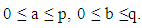 For the optimum model we are using the criteria of lower Akaike (AIC) and Schwartz (SIC), lower volatility as well as more significant coefficients.Thirdly, appropriate model estimation, involves the white noise terms in an ARIMA model. This entails a nonlinear iterative process in the estimation of the parameters. Maximum likelihood estimation is generally the preferred technique.Fourth, diagnostic checking of the appropriate model. This involves investigating whether the estimated model is acceptable and statistically significant, i.e. if it fits well to the data. According to Box and Jenkins for the adequacy of the estimated ARIMA model suggested checking the randomness of the residuals, i.e. whether the residuals from the estimated ARIMA model is white noise and are not serially correlated.Last but not the least, forecasting. One of the main reasons of the analysis of time series models is forecasting. The accuracy of the forecasts depends on the forecasting error. Moreover, some statistical measures are employed for this aim, such as root mean squared error (RMSE), mean absolute error (MAE), and mean absolute percentage error (MAPE) and the inequality coefficient of Theil (U). Then the forecast value one period ahead conditional on all information up to time, t, given at time t+k, [13] as:
 | (2) |
4. Econometric Results and Discussion
The variable used in the analysis is total unemployment (%) of the total labour force) that span from 1991 to 2019. The source of data is the World Bank Development Indicators (Online) [1]. The ARIMA approach is an iterative four-stage process of stationary testing, identification procedure of suitable model, estimation of the model and diagnostic checking and forecasting.
4.1. Testing Stationarity
Figure 1: Line graph of total unemployment (Raw data), shows a line graph of total unemployment, indicating no reversions to the mean (not stationary). The line graph shows a downward trend.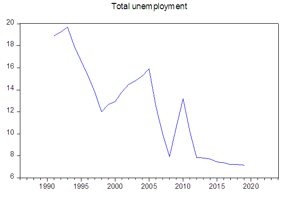 | Figure 1. Line graph of total unemployment (Raw data) |
Furthermore, Figures 2 and 3 represent the correlogram of total unemployment series with a pattern of up to the 12 lags in level and for first differences.Figure 2: Correlogram of total unemployment (Level) conclude that the coefficients of autocorrelation (ACF) starts with a high value and declines slowly, indicating non-stationary. Additionally, this (Figure 2) correlogram above also shows, the autocorrelation bars in both PACF and ACF that are statistically significant but outside the dotted standard error bound of 95%. Thus, the series must be configured in first differences.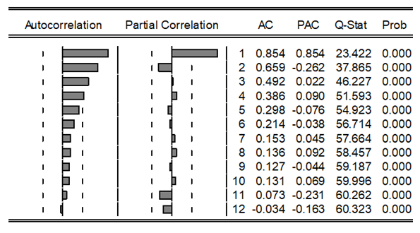 | Figure 2. Correlogram of total unemployment (Level) |
From Figure 3: Correlogram of Total Unemployment (First Difference) above, this paper observes that, coefficients of autocorrelation (ACF) starts with a high value and declines rapidly, indicating that the series is stationary. 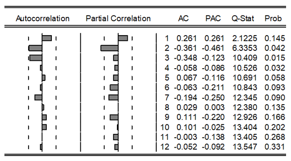 | Figure 3. Correlogram of Total Unemployment (First Difference) |
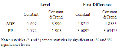
Table 1. ADF and Philip-Perron's Test
 |
| |
|
The stationarity test results in Table 1: ADF and Philip-Perron's Test, show that total unemployment will be of Integrated Order 1. Therefore, for our model ARIMA (p, d, q) we will have the value d=1.
4.2. Identification Procedure of the Model
We can use the correlogram of figure 3 to determine the values of parameters p and q in model ARMA (p, q). Regarding the aforesaid, an AR(p) model has a PACF that truncates at lag p and an MA(q)) has an ACF that truncates at lag q. In practice  are the non-significance limits for both functions. We shall explore the range of models ARMA (a, b):
  for an optimum one. To do this we shall use the automatic model determination criteria AIC and SIC. The limits for both functions (ACF, PACF) are
  Figure 3: Correlogram of Total Unemployment (First Difference), shows that, ACF cuts off at lag 4 (p=4) and the PACF at lag 1 (q=1). Exploring the range of models {ARMA (p, q):
  for the optimal based on AIC and SIC. Thereafter we create Table 2 with the values of p and q.
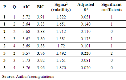
Table 2. Comparison of Models within the Range of Exploration using AIC,SIC,Sigma Square and Adjusted R-Squared
 |
| |
|
The results from Table 2: Comparison of Models within the Range of Exploration using AIC,SIC,Sigma Square and Adjusted R-Squared, above indicate that, according to the criteria of both lowest Akaike (AIC) and volatility (Sigma squared), ARMA model is formulated to ARMA (3,2). This model selected has also the highest adjusted R-Squared and a greater number of statistically significant coefficients. And since the model is stationary on first differences, i.e. (d=1) our ARIMA model will be ARIMA (3,1,2).
4.3. Estimation of the Model
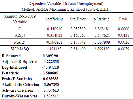
Having established the suitable econometric model as ARIMA (3,1,2), Table 3 shows the results of this model.The chosen model as summarized in Table 3 is ARIMA (3,1,2) and is given by: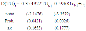 | (3) |
Both AR and MA coefficients are statistically significant at 5% and 1% level of significance respectively, as indicated by the results in Table 3. Additionally, Table 3 shows the non-linear techniques used by Eviews 10, which involved an iterative process that is converged after 16 iterations.Figure 4, shows the inverse roots of AR and MA characteristic polynomials for the stability of the ARIMA model (3,1,2). The corresponding inverse roots of the characteristic polynomials are stable since all the roots are in the unit circle indicating stationarity and invertibility respectively.Table 3. Estimation of Model (3,1,2)
 |
| |
|
 | Figure 4. Inverse Roots of AR and MA |
4.4. Diagnostic Checking of the Model
This paper use Q statistic of Ljung-Box [16] and Jarque Bera (JB) test [17] as a diagnostic test for autocorrelation and normality of the selected model (3,1,2). If the estimated model passes the two tests, it means the residuals are not auto correlated and follow normal distribution. 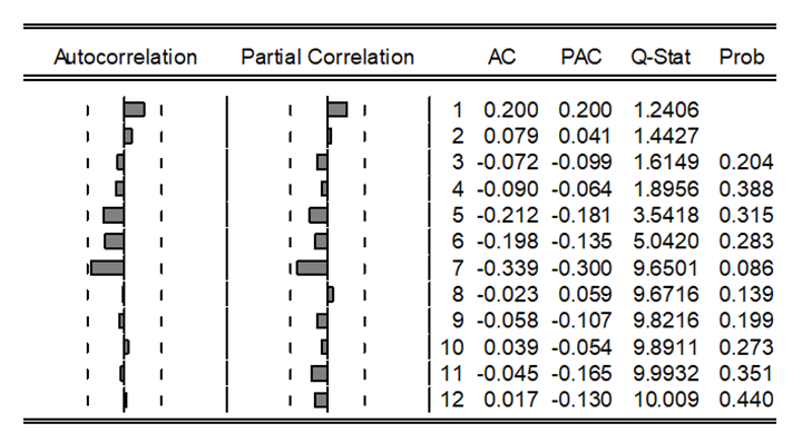 | Figure 5. Correlogram Q-statistics of ARIMA (3, 1, 2) |
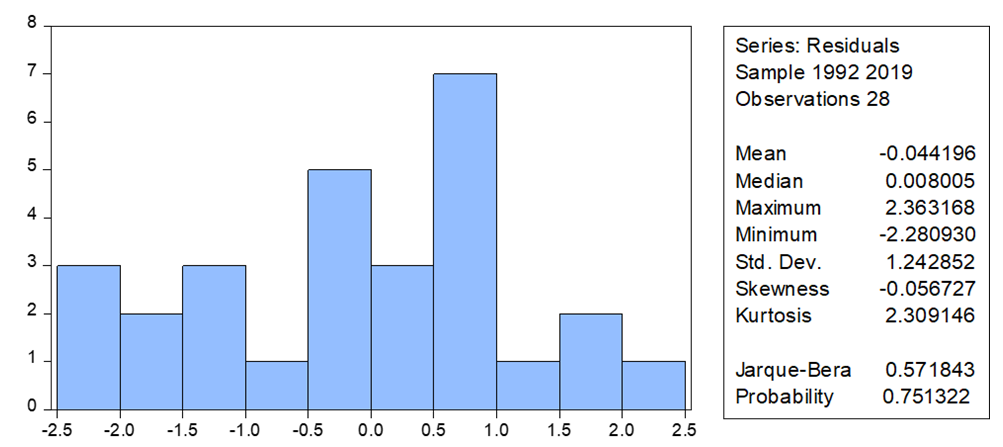 | Figure 6. Histogram of the residuals of the model ARIMA (3,1,2) |
The Figure 5: Correlogram Q-statistics of ARIMA (3, 1, 2) shows no missing information in the model since all the lags lie within the standard bounds (Dotted lines). Additionally, the Q statistic of Ljung–Box for all the 12 lags has values greater than 0.05 thus the null hypothesis cannot be rejected i.e. there is no autocorrelation for the examined residuals of the series.Normality test in Figure 6: Histogram of the residuals of the model ARIMA (3,1,2) shows that the residuals of ARIMA (3, 1, 2) model, follow a normal distribution.
4.5. Forecasting
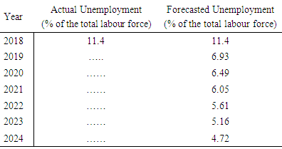
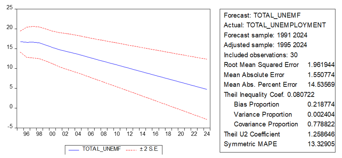
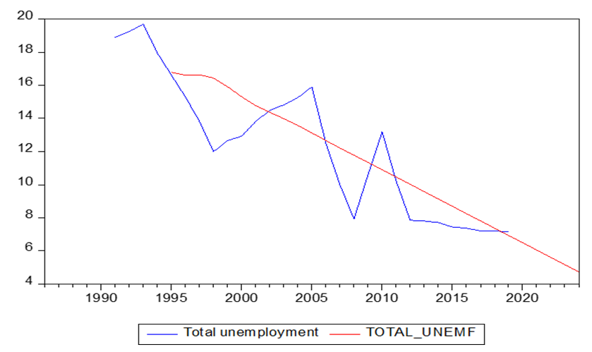
In figure 7, the paper represents the criteria for the evaluation of the forecasts of the model ARIMA (3,1,2). The results in figure 7 indicate that the forecast graph is within the standard bounds. The inequality coefficient of Theil has a lower value U1 = 0.0807 which means that our model has a good forecasting ability. Figure 8, which is, the plot of forecast Total unemployment graph against actual total unemployment shows how the forecast is closer to the actual values. The forecast shows a slowly and steadily declining trend.Table 4: Total unemployment Forecasts, summarizes the forecasting results of the Total unemployment over the period 2019 to 2024.Table 4. Total unemployment Forecasts
 |
| |
|
 | Figure 7. Forecast Accuracy Test on the Model ARIMA(3,1,2) |
 | Figure 8. Plot of forecast graph against actual (unemployment) |
5. Conclusions
Using the Box – Jenkins (B-J) Methodology, this paper is trying to forecast the total unemployment rate in Zambia for the next Five (5) years with an ARIMA model. The annual data of total unemployment rates used span from 1991 to 2019. After checking for the stationarity of the annual data series, the corresponding correlogram helped in choosing the appropriate p and q for the appropriate ARIMA (p, d, q) process. An ARIMA (3,1,2) model was created through the data used and estimating this model, we found that the total unemployment rate for the years 2020, 2021, 2022, 2023 and 2024 is forecast to be 6.49%, 6.05%, 5.61%, 5.16 and 4.72% respectively. That is, the trend of total unemployment in Zambia has been projected to be reducing steadily during the period under review. In this paper, unemployment is defined using three-fold guiding principles, namely: (a) not employed (b) not actively searching and (c) not available for work. This three-fold criterion distinguishes, those in the labour force from those who are not. According to the Zambia Demographic Survey of 2018, Zambia has a large population that does not meet the criterion. This explains why 6,154,252 persons of the 9,483,400 working-age population are outside labour force. The majority that meets criteria set for being in labour force or economically active (3,329,142 people as of 2018) are employed, leaving only 381,176 persons as unemployed. The total unemployment rate for 2018 was 11% (National Estimates). It is also important to bear in mind that, the economically active population (in absolute terms) shall keeping increasing, as the total population grows, every year. In relative terms the total unemployment rates may decline but in absolute terms, the number of the under employed or/and unemployed, arising from the projected share of the labour force may increase. That is assuming a smooth transition of working-age group into labour force. Nevertheless, deducing from a wider base of the Zambian population pyramid (a large young working-age population), the steady decline of projected total unemployment rates has future implications. That is, if the total unemployment rates has to reduce steadily from 2020 to 2024, it would mean, the number of Potential labour force (i.e. those outside the labour force), in absolute terms, would continue to increase over the period. The main plausible reasons for an increase in the potential labour force could be due to: Firstly, an increase in the number of those attending college or training. This paper is of the view that, in the next five (5) years, for the total unemployment to steadily reduce, there is likelihood of increased population of those not meeting the criteria to be considered in labour force and ultimately not considered unemployed. These young people in training and school are neither available nor actively searching for work, by strict operational definition of unemployment. Secondly, for total unemployment to reduce over time, it would also mean, majority young men and women would resort to working without pay or profit. Also Zambia has a substantially younger women population, family responsibilities of these women of the working-age might pull out of the labour force, among many other reasons. Or simply discouraged to actively participate due to stiff competition. This will closely be related to slow economic growth and few employment opportunities, bringing about competition for those who should stay in the labour market. This increases the potential labour force and reduces the unemployment rate. Lastly, failure to account for the proportion of the informal sector that passes the criteria of being part of labour force, would continue to contribute to Zambia’s under estimation of labour force as well as those unemployed. Zambia has a large informal sector. This line of thought justifies the steady decline in total unemployment but an increasing number of people outside the labour force. Reflecting on the results of this study will be helpful for the policy makers to formulate effective policies for attaining Sustainable Development Goal of providing decent working conditions for all Zambians. Zambia’s policy framework should not only focus on right classification of the actual labour force (employed and unemployed by operational guidelines provided) but also find ways to encourage large working-age population for smooth transition into the country’s labour force. The encouragement would be in form of increasing incentives for the potential labour force to swiftly consider being on the job market (More job opportunities). This paper is of the view that the decline in total unemployment rate observed in the forecast through historical data, is purely due to an increased number of those outside labour force in the next five years. Working on a true reflection of Country’s labour force and extent of unemployment shall help in policies that will reduce future youth unrest. This paper recommends that the 2020 Zambian census, should carefully address this issue. This paper also proposes further research on the unemployment forecast among education strata, i.e. separate projection on those with basic education, immediate education and advanced education. Since those are affected differently in the total labour force, in terms of finding jobs. Furthermore, the findings of the study will also help the Business Executives in managerial positions. Lack of new entrants in the labour market due to an increased number of the potential labour force, who are not willing and able to join labour force, humpers’ innovation. Reduced innovation, reduces the productivity and profitability of businesses.
Notes
1. In Zambia, the minimum age of persons in the working age population is 15 years. From the working age population two main categories are derived mainly the population Labour force and population outside the Labour force.2. Family responsibility are common among women. Women suffer more from discrimination and from structural, social, and cultural barriers that impede them from seeking work. Also, women are often responsible for the care of children and the elderly and for household affairs.
References
| [1] | World Bank Development Indicators (2019). Available at: https://databank.worldbank.org/source/world-development-indicators (Accessed: 4 December 2019). |
| [2] | International Labour Organization (2018), ‘Measuring Unemployment and the Potential Labour Force in Labour Force Surveys: Main findings from the ILO LFS pilot studies’, ILO Department of Statistics –Geneva, Switzerland (2018). Available at http://suo.im/6a9Rj7 (Accessed on 25 July 2020). |
| [3] | Central Statistical Office (2018), ‘Zambia Labour Force Survey Report’ [Online]. Available at: https://www.zamstats.gov.zm (Accessed: 10 December 2019). |
| [4] | Lusaka Times, (2020) ‘Zambia Police Warns Youth Planning to Conduct an illegal protest today, [online]. Available at: https://www.lusakatimes.com/2020/06/08/zambia-police-warns-youth-planning-to-conduct/ (Accessed: 26 July 2020). |
| [5] | Box, G. E. P. & Jenkins G. M. (1976).’Time series analysis. Forecasting and control’. Holden-Day, San Francisco. |
| [6] | International Labour Organization, ILOSTAT database. Data retrieved in September 2019.Social Protection & Labor: Unemployment. |
| [7] | Jovanovic, B. & Petrovska M. (2010). ‘Forecasting Macedonian GDP: Evaluation of different models for short-term forecasting’. Working Paper, National Bank of the Republic of Macedonia. |
| [8] | Zakai, M. (2014). ‘A time series modeling on GDP of Paki-stan’. Journal of Contemporary Issues in Business Re-search, 3(4), 200-210. |
| [9] | Mayor. M, Lopez, A. J. & Perez, R. (2007) ‘Forecasting Regional Employment with Shift–Share and ARIMA Modelling’, Regional Studies, 41:4, 543-551, DOI: 10.1080/00343400601120205. |
| [10] | Chakravarty, A. (2012) ‘The US Unemployment Rate: Stationarity’s Effect and Forecasting’, Academia. edu, volume (issue/season). |
| [11] | Claveria, O. (2019). ‘Forecasting the unemployment rate using the degree of agreement in consumers’ expectations. 13th ifo Dresden Workshop on Macroeconomics and Business Cycle Research (Dresden, January 25-26, 2019), AQR-IREA, University of Barcelona (UB). |
| [12] | Hyndman, R.J. and Khandakar, Y. (2008) ‘Automatic time series forecasting: The forecast package for R’. Journal of Statistical Software, 27(3), 1–22. |
| [13] | Dritsaki, C. (2015) ‘Forecasting Real GDP Rate through Econometric Models: An Empirical Study from Greece.’, Journal of International Business and Economics, Vol. 3, No. 1, pp. 13-19 ISSN: 2374-2208 (Print), 2374-2194 (Online). Available at: URL: http://dx.doi.org/10.15640/jibe.v3n1a2. |
| [14] | Dickey, D. A. & Fuller W. A. (1979). ‘Distribution of the estimators for autoregressive time series with a unit root’. Journal of the American Statistical Association, 74(366), 427–431. |
| [15] | Phillips, P. C. B. & Perron P. (1988). Testing for a unit root in time series regression. Biometrika, 75(2), 335–346. |
| [16] | Ljung, G. M., & BoxG. E. P. (1978). ‘On a measure of a lack of fit in time series models’. Biometrika, 65(2), 97–303. |
| [17] | Jarque, C. M., & Bera A. K. (1980). Efficient tests for normality, homoscedasticity and serial independence of regression residuals. Economics Letters 6(3), 255–259. |

 Abstract
 Reference
 Full-Text PDF
 Full-text HTML