Zaher Khraibani1, 2, Hussein Trabulsi3, Alya Atoui1, 4, Ali Hayek4, Dana Radwan2
1Environmental Physio-Toxicity group, Rammal Hassan Rammal laboratory, Lebanese University, Faculty of Sciences, Nabatieh, Lebanon
2Lebanese University, Faculty of Sciences, Department of Appliad Mathematics, Hadat, Lebanon
3Department of Economics, Faculty of Economic Sciences & Business Administration, Lebanese University, Beirut, Lebanon
4Laboratoire Eau, Environnement et Systèmes Urbains (LEESU), Université Paris Est, France
Correspondence to: Zaher Khraibani, Environmental Physio-Toxicity group, Rammal Hassan Rammal laboratory, Lebanese University, Faculty of Sciences, Nabatieh, Lebanon.
| Email: |  |
Copyright © 2020 The Author(s). Published by Scientific & Academic Publishing.
This work is licensed under the Creative Commons Attribution International License (CC BY).
http://creativecommons.org/licenses/by/4.0/

Abstract
As agriculture is considered one of the most important economic sectors in Lebanon, the aim of this article is to study the impact of precipitation and temperature on economic growth through agriculture in Lebanon. In addition, the presence of climate change in the developing countries, in the Mediterranean region which has been considered a place of transition between two large climatic units, becomes certainty and represents an ecological, economic and social threat. This analysis is made with an autoregressive VAR model, between time series variables, based on the stationarity test. The results show the presence of two models, long and short term models that explain the direct positive effect of precipitation and the direct and indirect effect of temperature on the GDP of agriculture in Lebanon with a non-significant effect for the short term period.
Keywords:
Precipitation, Temperature, VAR model, GDP, Agriculture, Lebanon
Cite this paper: Zaher Khraibani, Hussein Trabulsi, Alya Atoui, Ali Hayek, Dana Radwan, Climate Change, Agriculture and Economic Growth in Lebanon: A VAR Approach, American Journal of Economics, Vol. 10 No. 3, 2020, pp. 126-131. doi: 10.5923/j.economics.20201003.02.
1. Introduction
The variation of the climatic conditions of the environment such as humidity, temperature, rainfall, or carbon dioxide content, results in a geographical shift of the habitats in which the animal and plant species can live. It will modify the possible growing and cultivation types in each region. Since the beginning of the Eath's life, the climate has constantly undergone "natural" changes due to volcanoes, floods, drought, deterioration of the ozone layer, and the natural emission of carbon dioxide. These changes have been aggravated following the appearance of humans, drawing more and more natural resources, more especially by industrial activity.Almost all Lebanese territory is under the influence of the Mediterranean climate, characterized by heavy winter rains and summers without rain, separated by very short transition seasons, spring and autumn. The agricultural sector is basic for the economy and social development in many Arab countries, especially Lebanon. Agriculture in Lebanon is considered one of the most important financial sectors.The loss caused by climate change is threatening the agricultural sector in Lebanon, thus increasing the unemployment rate and declining the GDP, because of the absence of climate forecasts and the necessarily required statistics to develop certain strategies to decrease their negative effects.Several numerical models have been developed by the scientific community in order to establish detailed estimates of all possible responses of the impact of several factors on the GDP of agriculture integrating the temperature, the precipitation, the employment, the capital, the agriculture production index [1], [2], [3]. Indeed, the literature on climate change impacts on agriculture has been dominated by two different methodologies. One method applies static econometric models to time series, cross-sectional, or panel data, whereas the second one uses the Ricardian or hedonic method derived from Ricardo (1817) as a theoretical background. We mention some of them for illustration purposes: [4], [5], [6], [7], [8].Thus, the purpose of our work is to study the impact of climate change on growth through agriculture over the last 23 years, through an econometric VAR (Vector autoregression) model that analysis a couple of climatic variables (temperature and precipitation), the agricultural yield and the GDP.
2. Materials and Methods
2.1. Variables Description
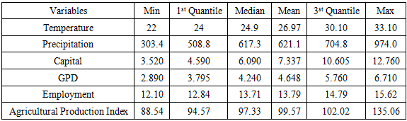
The different variable available in the data of 23 observations collected annually:- Years: from 1996 until 2018- Temperature: the average temperature of each year from 1996 till 2018- Precipitation: the total rainfall of each year form 1996 till 2018- Capital: the proportion of income saved and invested by farmers- GDP: Growth domestic product coming from the agricultural sector- Employment: persons of working age who were engaged in any activity to produce goods or provide services (in percentage)- Agricultural Production Index: shows agricultural production for each year relative to the base period 1996-2018. Table 1. Descriptive Statistics for VAR model Variables
 |
| |
|
The agricultural sector contributes about 4% of GDP, representing 6% of national employment and it provides for about 15% of income for the population. However, climate change and the consequential risks increase year by year and contribute to the elimination of 20 to 40 percent of crops annually and increase in the loss of the agricultural sector resulting from the risks produced by the climate change that is unable to be adapted.Thus, we can have our first perspectives from figures 1 and 2, where the impact is positive for the relation of the value of agriculture and the precipitation and it is negative for the relation of agriculture and the temperature. As seen in the two graphs above, when the amount of rain is increasing, we deduce an increasing in the value of agriculture for the next season, which is the opposite of the temperature.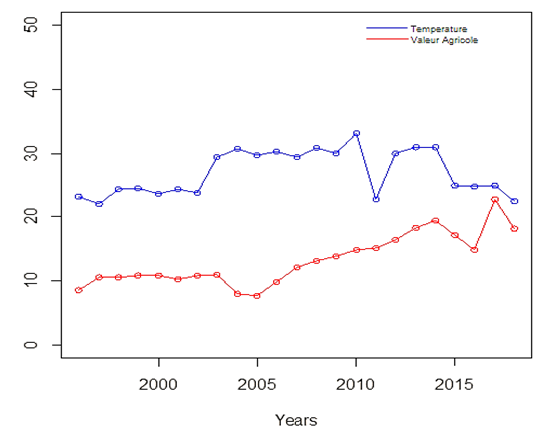 | Figure 1. Evolution of the temperature and the agricultural value |
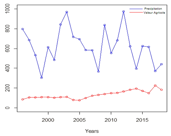 | Figure 2. Evolution of the precipitation and the agricultural value |
What we are looking to verify in the upcoming part, is the estimation of the econometric model of the GDP in function of the climatic variables. The model of our work is based on an approach of terms of production which build a relation between the GDP (Y) in function of the capital (K), employment (L), agricultural production index (Ia) and a climate change indicator (CC). This model is close to the model used by Cobb Douglass production function, defined as follows: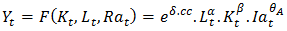 Where
Where 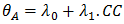 When substituent the second equation in the first one, we obtain:
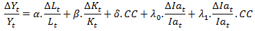 Our model is divided into two models. In the first model, we will use the variable precipitation (P) as an indicator of the level climatic change and in the second model, this level is measured from the temperature (T). Thus the two models expressed in log, to make are variables at the same level, are specified as follows:
 Where,
  is the error.Differently with other models, the VAR model allows studying the relations between different time series at once (precipitation or temperature, agricultural production index and the GDP), which allow us to simultaneously take the direct and indirect impact of climatic changes on economic growth.
 measure the direct effect of the climatic changes on the economic growth, while
  measure the effect of the climatic changes on economic growth via agricultural.
3. Results and Discussion
The econometric method used in this article is based on three steps: first we test the unit roots using the test that is proposed by . Then we perform the tests proposed by to obtain the long-term relationship between all the variables. Finally, we apply the modified OLS technique (MOLS) to estimate the co-integration vector of co-integrated heterogeneous panels.According to figure 3, the shape of the curves of GDP, employment, capital, agricultural production index, and temperature and precipitation, have a general tendency either to downward or upward. Their assessments over time, show a unique and ascending tendency, which puts their stationarity into levels, this leads us to the stationarity test to check the existing of root unit, and by using the augmented Dickey-fuller test (ADF), then we test the existence of co-integration relation between the variable to determine the order of the VAR model (Autoregressive model) to estimate the model.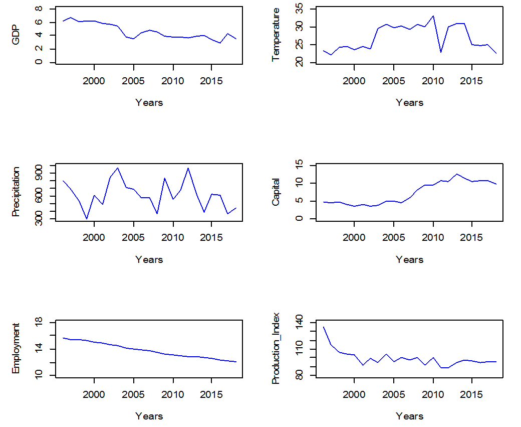 | Figure 3. Graphs of variables |
Estimation of model 1:Table 2. Differentiation Test of Model 1
 |
| |
|
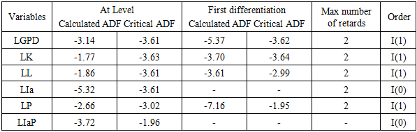
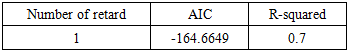
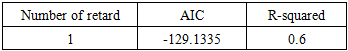
Stationarity of variables: From table 2, we note that the variables (LGDP, LK, LL, LP) have an ADF less than the critical values, but after the first differentiation, they become significant, thus the variables with order equal to 1 (I(1)) are integrated in the model. Then, we can conclude that the co-integration relation may exist.To verify the existence of such a relation between the retained variables, there are two stages to follow. First, we have to determine the optimal number of retards for the model. Secondly, we will use the test of Johnson to detect the number of co-integration relations between the variables.Choice of retard number:To choose the size of a VAR model of order p (starting from 0 to a fixed order h). We use the information criteria AIC. The choice of the number of retards has an important role in the estimation of the VAR model. We choose the model which has the minimum AIC. Table 3. Number of Retard of Model 1
 |
| |
|
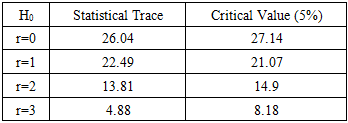
Table 3 shows that the number of retards is equal to 1, since the AIC criteria is minimum for this number of retard. Test de Johansen:This test gives the number of cointegration relations between the existed variables for the long term. Thus, we use this method of maximum likelihood where the results are shown in Table 4.Table 4. Johansen Test for Model 1
 |
| |
|
To determine the number of co-integration relation between the variables, we test the above hypothesis H0.If the calculated value > critical value, we reject the null hypothesis of absence of co-integration relation. Thus, there is at least one co-integration relation and the model is retained.Model 1:The equilibrium relation of long term: After the estimation of the long term model, we will estimate in the following the model of correction error:
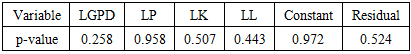
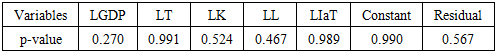
 Results of the estimation:It is obvious that in the long term model, there exists a positive significant relation between the capital, the employment and the precipitation with the economic increasing throughout the agriculture.The results of this estimation show that if the precipitation increases of 1%, it will causes an increasing of 3.43% of the GDP.For the short term model, the p-values in table 5 are bigger than 0.05 thus the variable are not significant enough to take them into consideration for a short term model. In this case we cannot discuss the economical results of this model.
Table 5. Test of Student for Model 1 (Short)
 |
| |
|
Estimation of model 2:Same method is applicable as above. First we test the stationarity of the two remaining variables.Table 6. Differentiation Test of Model 2
 |
| |
|
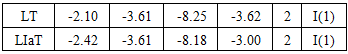
From table 6, we conclude that the two variables LT and LIaT are stationary after one differentiation and of the same cointegration order. Thus the long term model exists containing the following variables (LGDP, LK, LL, LT, LIaT).Choice of retard number:Table 7. Number of retard of Model 2
 |
| |
|
Same as the model 1, the number of retards is equal to 1 as shown in table 7.Test de Johansen:This test gives the number of co-integration relation between the existed variables for a long term. Thus, we use this method of maximum likelihood; the results are shown as follows:Table 8. Johansen Test for Model 2
 |
| |
|
The table 8 shows that also in the model 2 the number of co-integration relation is at least equal to one, because the calculated value for r≤2 is less than the critical value.Model 2:The equilibrium relation of long term: After the estimation of the long term model, we will estimate the model of correction error:
 Results of the estimation:In the long term model with temperature taken as the climatic index, it shows that the direct and indirect effect of temperature has a negative evolution on the GDP. An increase of 1% in temperature will lead to a decreasing of 0.03% in the GDP. This explains the effect of temperature for long the term can affect not only the agriculture sector, but also the tourism, and public health since it can increase the diseases.The results of this estimation show that if the precipitation increases of 1%, it will cause an increase of 3.43% of the GDP.For the short term model, the p-values shown in table 9, are bigger than 0.05, thus the variables are not significant enough to take them into consideration for a short term model. In this case, we can’t discuss the economical results of this model.
Table 9. Test of Student for Model 2 (Short)
 |
| |
|
The results of the second model allowed us to see the negative direct and indirect effects of temperature on economic growth. But in the short term model, as the p-values are bigger than 0.05, then the variable in this model are not significant and for a short period, the temperature doesn’t have any effect on the economic growth.
4. Conclusions
The climatic change is one of the major sources of concern in our century. In this thesis with a VAR model, we showed the effect of the evolution of temperature and precipitation, as principle factors in the climatic change, on the GDP in the agricultural sector.The results of these estimations show that after one differentiation by taking the stationary variable, these variables are significant for the long term and affect the economic growth in the upcoming long period. It seems that the precipitation has a positive effect on the economic growth, while the temperature has a negative effect i.e. the increasing in precipitation and decreasing in temperature will affect positively on the agricultural sector and thus on the economic growth.
References
| [1] | M. S. F. N. T. H. v. V. Günther Fischer, "Socio-economic and climate change impacts on agriculture: an integrated assessment, 1990–2080," Philos Trans R Soc Lond B Biol Sci., p. 2067–2083, 2005. |
| [2] | S. A. W. Syed Ali Fazal, "Economic Impact of Climate Change on Agricultural Sector: A," Economic Impact of Climate Change on Agricultural Sector: A, pp. 39-49, 2013. |
| [3] | Ching-ChengChang, "The Potential Impact of Climate Change on Taiwan’s Agriculture," Agricultural Economics, pp. 51-64, 2002. |
| [4] | K. T. A. J. Lippert C., " A Ricardian analysis of the impact of climate change on agriculture in Germany," Climatic Change, pp. 593-610, 2009. |
| [5] | M. G. Deschênes Olivier, "The Economic Impacts of Climate Change: Evidence from Agricultural Output and Random Fluctuations in Weather: Reply," American Economic Review, vol. 102, no. 7, pp. 3761-3773, 2012. |
| [6] | H. M. F. C. Schlenker W., "Will U.S. agriculture really benefit from global warming? Accounting for irrigation in the hedonic approach," American Economic Review, vol. 95, pp. 395-406, 2005. |
| [7] | H. B. L. S. L. N. Adams R., "Effects of global climate change on world agriculture: an interpretive review," Climate Research, vol. 11, pp. 19-30, 1998. |
| [8] | T. F. G. R. B. J. Rosenzweig C., "Increased crop damage in the US from excess precipitation under climate change," Global Environmental Change, vol. 12, pp. 197-202, 2002. |
| [9] | M. PESARAN, "A simple panel unit root test in the presence of cross section," Journal of Applied Econometrics, vol. 22, p. 265–312, 2007. |
| [10] | J. WESTERLUND, "Testing for error correction in panel data," Oxford Bulletin of Economics and Statistics, vol. 69, no. 6, p. 709–748, 2007. |
| [11] | O. Zouabi, "Climate Change, Impacts on Agriculture," Munich Personal RePEc Archive, p. 19, 2015. |
| [12] | P. Tissot, "L'Agriculture libanaise: son présent et son avenir.," Journal d'agriculture traditionnelle et de botanique appliquée, pp. 110-119, 1947. |
| [13] | F. E. Harrell, "Regression modeling strategies," As Implemented in R Package ‘Rms’ Version, p. 3(3), 2014. |
| [14] | H. Hamisultane, "Modéle à correction d'erreur (MCE) et applications," 2002. [Online]. Available: https://halshs.archives-ouvertes.fr/cel-01261167. |

 Abstract
 Reference
 Full-Text PDF
 Full-text HTML