Salah H. Abid
Mathematics Department, Education College, Mustansiriyah University, Iraq
Correspondence to: Salah H. Abid, Mathematics Department, Education College, Mustansiriyah University, Iraq.
| Email: |  |
Copyright © 2019 The Author(s). Published by Scientific & Academic Publishing.
This work is licensed under the Creative Commons Attribution International License (CC BY).
http://creativecommons.org/licenses/by/4.0/

Abstract
In this paper, vector autoregressive model (VAR) is used to represent the most important variables in the Iraqi economy which are, Foreign Investment (FI), Iraqi Investment (II), Imports (IM), Exports (EX), Expenses (EXP), Income (IN), Broad Money (M2), Oil price (OI), Gross Domestic Product In Constant Price (2007=100) (GDP), Gross Foreign Assets of CBI (GF) and Exchange Rate in market price (ER). VAR model is estimated and some related tests are conducted. As a result, small model for economy of Iraq is obtained. To complete the work, principal component analysis is used for policy-making and prioritization for economy of Iraq. Most of information, approximately 86.13, is contained in three factors only. Based on the obtained results, all plans, policies and programs of economic and development in Iraq must be made according to the effects of factors and consequently variables under consideration.
Keywords:
Vector autoregressive model (VAR), Principal component analysis, Stability, Wald Test, Semi-simulated data, Akaike information criterion (AIC), Schwarz information criterion (SC)
Cite this paper: Salah H. Abid, Small Model for Economy of Iraq Based on Semi-simulated Data, American Journal of Economics, Vol. 9 No. 5, 2019, pp. 242-258. doi: 10.5923/j.economics.20190905.03.
1. Introduction and Work Aims
The VAR model was introduced by Sims (1980) as a method to analyze macroeconomic data. He developed the VAR model as an alternative to the traditional system, which involved several equations.Athanasopoulos et al in 2010 studied the joint determination of the lag length, the dimension of the cointegrating space and the rank of the matrix of short-run parameters of a vector autoregressive (VAR) model using model selection criteria. They considered model selection criteria which have data-dependent penalties as well as the traditional ones. They suggested a new two-step model selection procedure which is a hybrid of traditional criteria and criteria with data-dependant penalties and they proved its onsistency. Their Monte Carlo simulations measure the improvements in forecasting accuracy that can arise from the joint determination of lag-length and rank using their proposed procedure, relative to an unrestricted VAR or a cointegrated VAR estimated by the commonly used procedure of selecting the lag-length only and then testing for cointegration. Two empirical applications forecasting Brazilian inflation and U.S. macroeconomic aggregates growth rates respectively show the usefulness of the model-selection strategy proposed here. The gains in different measures of forecasting accuracy are substantial, especially for short horizons.Emmanuel in 2015 used the VAR models to model the Growth Domestics Products (GDP) of Ghana with other two selected macroeconomic such as inflation and real exchange rate for the period of 1980 to 2013. The empirical results derived, indicated that all the variables were stationary after their first differencing. The study further established that there is cointegration between macroeconomic variables and GDP in Ghana indicating long run relationship. The VECM (3) model was appropriately identified using AIC information criteria with co-integration relation of exactly one.Kononenko in 2015 used VAR Methodology as well as Vector Error Correction (VEC) methodology to examine the existence and direction of causality between economic growth and IMF lending for Ukraine. The paper examines the IMF lending data for the period of 1991-2010. Robust empirical analysis indicates that IMF lending has a negative effect of on Ukraine's economic growth in the short term. Policy implications of this finding are that, despite short-run decline in economic growth, IMF lending can result in a long-run sustainable growth for Ukraine. For this, policymakers need to ensure that fund's money are used not only to cover budget's deficit, but also to finance institutional reforms.Demeshko et al in 2016 characterized the relations of the discrete time domain DVAR model with its corresponding Structural Vector AR (SVAR) and Continuous Time Vector AR (CTVAR) models through a finite difference method across continuous and discrete time domain. They further clarified that the DVAR model of a continuous time, multivariate, linear Markov system is canonical under a highly generic condition. Their analysis shows that they can uniquely reproduced its SVAR and CTVAR models from the DVAR model. Based on these results, they proposed a novel Continuous and Structural Vector Autoregressive (CSVAR) modeling approach to derive the SVAR and the CTVAR models from their DVAR model empirically derived from the observed time series of continuous time linear Markov systems. They demonstrated its superior performance through some numerical experiments on both artificial and real-world data.Gudeta et al in 2017 investigated the effect of export and import on real economic growth of Ethiopia. Yearly data set on the variables are obtained for the period 1982 to 2015 from national bank of the country. VAR analysis suggests that the lagged variables of both export and import have significant contributions in predicting the economic growth of the country.In 2018, Forni et al resumed the line of research pioneered by Sims and Zha (Macroeconomic Dynamics, 2006, 10, 231–272) and make two novel contributions. First, they provided a formal treatment of partial fundamentalness, that is, the idea that a structural vector autoregression (VAR) can recover, either exactly or with good approximation, a single shock or a subset of shocks, even when the underlying model is nonfundamental. In particular, they extended the measure of partial fundamentalness proposed by Sims and Zha to the finite‐order case and study the implications of partial fundamentalness for impulse‐response and variance‐decomposition analysis. Second, they presented an application where they validated a theory of news shocks and found it to be in line with the empirical evidence.Huber and Pfarrhofer in 2019 provided a parsimonious means to estimate panel VARs with stochastic volatility. They assumed that coefficients associated with domestic lagged endogenous variables arise from a Gaussian mixture model. Shrinkage on the cluster size was introduced through suitable priors on the component weights and cluster-relevant quantities were identified through novel shrinkage priors. To assess whether dynamic interdependencies between economies are needed, they moreover impose shrinkage priors on the coefficients related to other countries’ endogenous variables. Finally, their model controls for static interdependencies by assuming that the reduced form shocks of the model feature a factor stochastic volatility structure. They assessed the merits of the proposed approach by using synthetic data as well as a real data application. In the empirical application, they forecast Eurozone unemployment rates and shows that their proposed approach works well in terms of predictions.Hecq et al in 2019 developed an LM test for Granger causality in high-dimensional VAR models based on penalized least squares estimations. To obtain a test which retains the appropriate size after the variable selection done by the lasso, they proposed a post-double selection procedure to partial out the effects of the variables not of interest. They conducted an extensive set of Monte-Carlo simulations to compare different ways to set up the test procedure and choose the tuning parameter. The test performs well under different data generating processes, even when the underlying model is not very sparse. They investigated also two empirical applications: the money-income causality relation using a large macroeconomic dataset and networks of realized volatilities of a set of 49 stocks. In both applications they find evidences that the causal relationship becomes much clearer if a high- dimensional VAR is considered compared to a standard low-dimensional one.Aikman in 2019 presented a methodology for modelling the interaction between quantiles of endogenous variables in a VAR. They apply this to a bivariate quantile VAR on euro area data for industrial production and a financial stress indicator. They find that financial shocks shift the shape of the distribution of industrial production in the short term, increasing the fatness of the tail.Owing to its simplicity and less restrictions, the vector autoregressive with exogenous variable (VARX) model is one of the statistical analyses frequently used in many studies involving time series data, such as finance, economics, and business. PTBA and HRUM energy as endogenous variables and exchange rate as an exogenous variable were studied by Warsono in 2019. The data used were collected from January 2014 to October 2017. The dynamic behavior of the data was also studied through IRF and Granger causality analyses. The forecasting data for the next 1 month was also investigated. On the basis of the data provided by these different models, it was found that VARX (3,0) is the best model to assess the relationship between the variables considered in this work.In this paper, we have two aims, the first one is the modeling of most important variables of Iraqi economy, model estimation and related issues. The second aim is the policy-making and prioritization for economy of Iraq.
2. VAR Process Model
The vector autoregression (VAR) is usually used for forecasting systems of interconnected time series and for analyzing the influence of random errors on the system of variables. VAR processes are common in economics because they are easy and ductile models for multivariate time series data. Var models became standard tools since Sims (1980) contested the way traditional simultaneous equations models were named, recognized and recommended these models as alternatives. These models are treated in depth in books of Lütkepohl (2005) and Hamilton (1994). VAR models does not need for structural modeling by considering every endogenous variable as a function of the lagged values of all of the endogenous variables in the system. Suppose that we interested in a set of  related time series variables collected in
  The mathematical form of a VAR model is,
 | (1) |
Where  is a
is a  vector of endogenous variables,
  are
are  matrices of parameters,
  is a vector of deterministic terms such as a constant, a linear trend and/or seasonal,
  is the matrix of parameters related with
  , and
, and  is a vector of errors that may be jointly correlated but are uncorrelated with their own lagged values and uncorrelated with all of the right-hand side variables. The error process
  is assumed to be white noise with zero mean, that is,
  , the covariance matrix,
  , is time invariant and the
  are serially uncorrelated or independent.By using the lag operator
  , (1) can be reformed as,
 | (2) |
The VAR process is stable if all roots of the determinantal polynomial are outside the complex unit circle, which is mean that,  for
for  Since that any stable process
  has time invariant means, variances and covariance structure and is, hence, stationary.VAR models are suited tools for forecasting. If the
  are independent white noise, the minimum mean squared error (MSE) h-step forecast of
  at time t is the conditional expectation given
 | (3) |
Where  for
for  Using this formula, the forecasts can be computed recursively for
  . The forecasts are unbiased, that is, the forecast error
 has mean zero and the forecast error covariance is equal to the MSE matrix. The one-step ahead forecast errors are the
  VAR models can also be consumed for analyzing the connections among variables involved. For example, Granger (1969) determined a notion of causality which given that a variable
  is causal for a variable
  if the information in
  is beneficial for ameliortating the forecasts of
  If the two variables are jointly generated by a VAR process, it turns out that
  is not Granger-causal for
  if a simple set of zero conditions for the VAR model coefficients are fulfilled. Hence, Granger-causality is light to check in VAR processes.
2.1. Estimation and Model Specification
Usually, in practical applications, the process which has generated the time series under study is unknown. So, if VAR models are considered as appropriate, the lag order has to be determined and the parameters have to be estimated. Consequently, for a given VAR of order p, estimation can be well done by the ordinary least squares (OLS). For a sample of size  and assuming that moreover initial values
  are available, the OLS estimator of the parameters
  will be,
 | (4) |
Where,  . Under standard assumptions the estimator is consistent and asymptotically normally distributed. Actually, if the residuals and, hence, the
  are normally distributed, that is,
  the OLS estimator is equal to the maximum likelihood (ML) estimator with the usual asymptotic optimality properties. It is well known that, the number of parameters is also large, when the dimension
  of the process is large, then the estimation precision may be low if a sample of typical size in macroeconomic studies is available for estimation. In that case, it may be opportune to use so-called subset VAR models by estranging excessive lags of some of the variables from some of the equations. Generally, other estimation methods may be more efficient if some restrictions are enjoined on the parameter matrices.By the following most popular model selection criteria, VAR order selection is usually done,1. Akaike’s information criterion (AIC) (Akaike, 1973), with the form,
 2. Hannan-Quinn criterion (HQC) (Hannan and Quinn, 1979), with the form,
 Where,
  is the residual covariance matrix of a
  model estimated by OLS. The VAR order is chosen which perfectly equipoises both terms. Factually, models of orders
  are estimated and the order
  is chosen such that it minimizes the value of the criteria.The fact that
  implies to that the
  generally chooses models with a smaller 𝑝 while AIC chooses models with a higher order 𝑝.Once a model is estimated it should be checked that it represents the data features sufficiently. If some of the time series variables to be modeled with a VAR have stochastic trends, that is, they manage similarly to a random walk, and then another model framework may be more suitable for analyzing especially the trending properties of the variables. Stochastic trends in some of the variables are generated by models with unit roots in the VAR operator, that is
  , for
, for  . Variables with such trends are nonstationary and not stable. They are often called integrated. They can be made stationary by differencing. Furthermore, they are called cointegrated if stationary linear combinations exist or, in other words, if some variables are driven by the same stochastic trend. Cointegration relations are often of specific benefit in economic studies. In that case, reparameterizing the standard VAR model such that the cointegration relations appear immediately may be appropriate. The so-called vector error correction model (VECM) of the form,
 | (5) |
is a simple example of such a reparametrization, where  denotes the differencing operator defined such that,
  ,
,  and
and 
 for
for  . This parametrization is acquired by subtracting
  from both sides of the standard VAR formulation and rearranging terms. Its merit is that
  can be decomposed such that the cointegration relations are straight sitting in the model. More accurately, if all variables are stationary after differencing once, and there are
  common trends, then the matrix
  has rank
  and can be decomposed as,
  , where
  and
and  are
are  matrices of rank
  and
and  includes the cointegration relations. A detailed statistical analysis of this model is offered in Johansen (1995).
3. Model of Iraqi Economy
In this section, a small model for economy of Iraq will presented according to data obtained from the website of central bank of Iraq. The variables used here are Foreign Investment (FI), Iraqi Investment (II), Imports (IM), Exports (EX), Expenses (EXP), Income (IN), Broad Money (M2), Oil price (OI), Gross Domestic Product In Constant Price (2007=100) (GDP), Gross Foreign Assets of CBI (GF) and Exchange Rate in market price (ER). The data shown in table (1) in appendix. Three of variables IM, EX and GDP have been compiled on an annual basis, while the other variables were compiled on a monthly basis. To unify these basis, we estimated three annual models based on time as independent variables to simulate the monthly values of these variables. The models are as follows, | (6) |
With adjusted determination coefficient  equal to 97.9491 and mean square error equal to 4.1018E7.
 | (7) |
With adjusted determination coefficient  equal to 93.9906 and mean square error equal to 248.287.
 | (8) |
With adjusted determination coefficient  equal to 99.1058 and mean square error equal to 229.995.Three models are accepted to represent data according to F-ANOVA test at all popular significant levels 0.01, 0.05 and 0.10. The simulated data are recognized by red color in table (1) and the variables which are simulated will recognized by letter s, to be GDPS instead of GDP, EXS instead of EX and IMS instead of IM. We will present our work according to the following steps,(1) The VAR model is considered. Table (1) shows the results of model estimation. The estimates of model parameters are in the first line at each of independent variables. The second line contains the standard deviation for each corresponding estimate while the third line contains the computed t- statistic to test the null hypothesis, which is said that the parameter under consideration is equal to zero, against the alternative hypothesis, which is not said that. The p-value is contained in the fourth line. The bold font for the p-values is used to recognize the rejected hypotheses, which is meaning that the variable has an effect. (2) The values of Adj. R-squared, Log likelihood, Akaike AIC and Schwarz SC in table (1), show that the model is worked well done.(3) The initial VAR model (which is contained all considered independent variables and lagged variables of order 2 according to criteria in table (2)) is as follows,
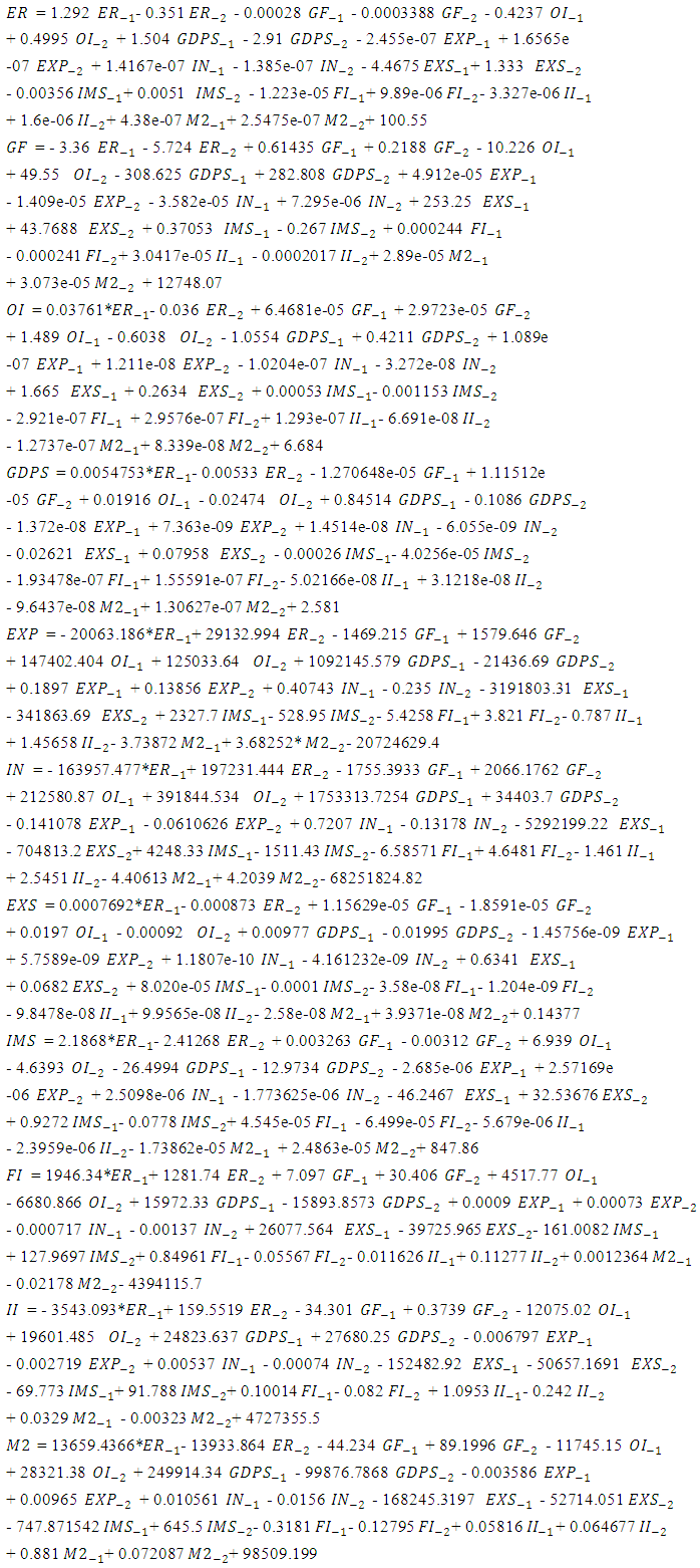 | (9) |
Graph (1) represent the residuals for each considered random variable,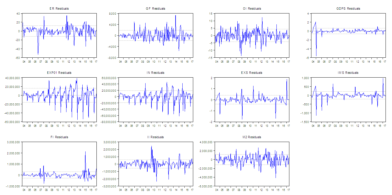 | Figure (1). Residuals for each considered random variable |
(4) According to the results of t-test in table (1) and Granger Causality/Block Exogeneity Wald Tests in table (3), the final VAR model (which is contained the effective independent variables only ) is as follows,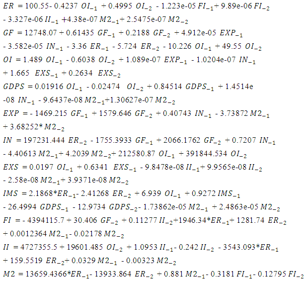 | (10) |
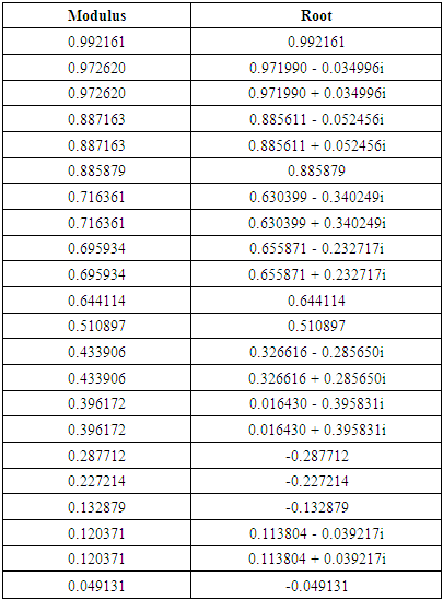
(5) According to the results in tables (4) and (5) and figure (2), It is clear that No root lies outside the unit circle, then VAR model satisfies the stability and consequently stationarity condition.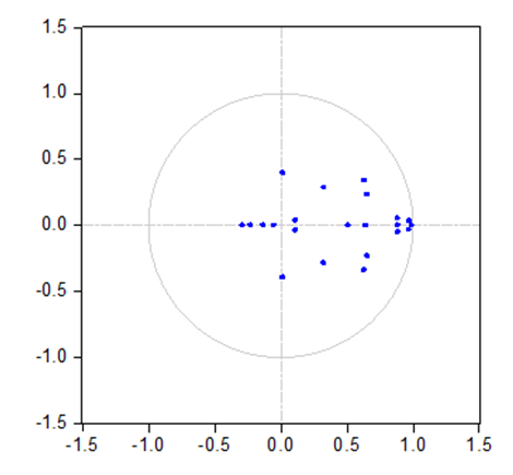 | Figure (2). Inverse roots of AR characteristic polynomial |
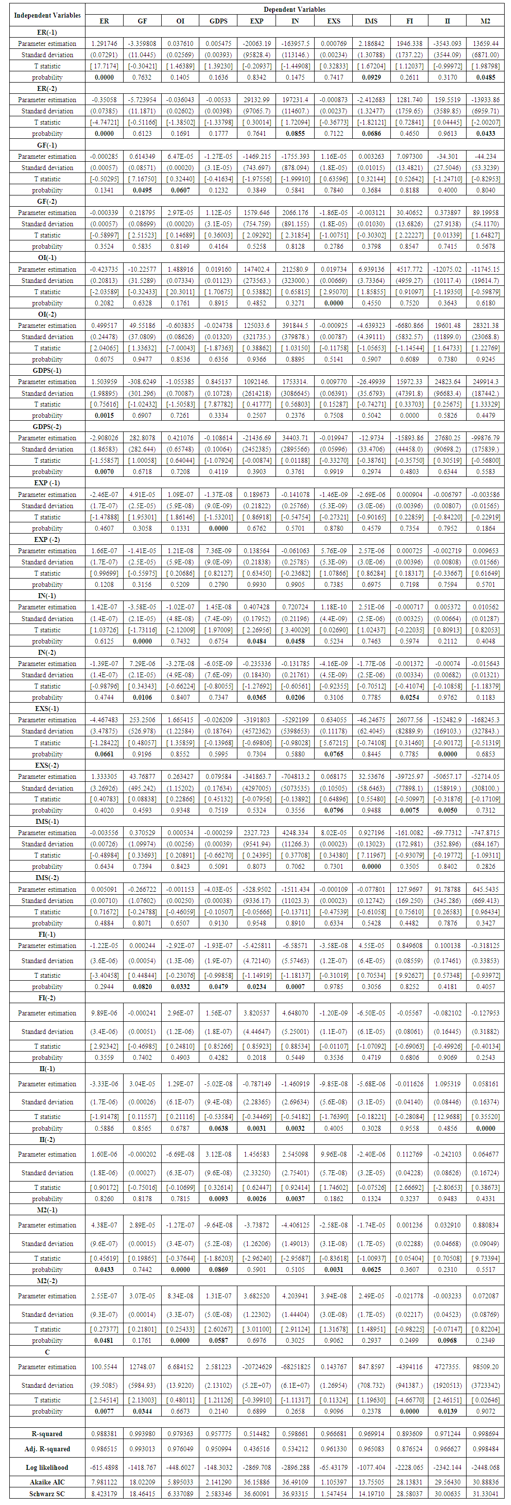 | Table (1). Shows the results of model estimation and evaluation |
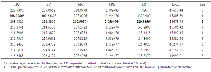 | Table (2). VAR Lag Order Selection Criteria for Endogenous variables ER, EXP, EXS, FI, GDPS, GF, II, IMS, IN, M2 and OI |
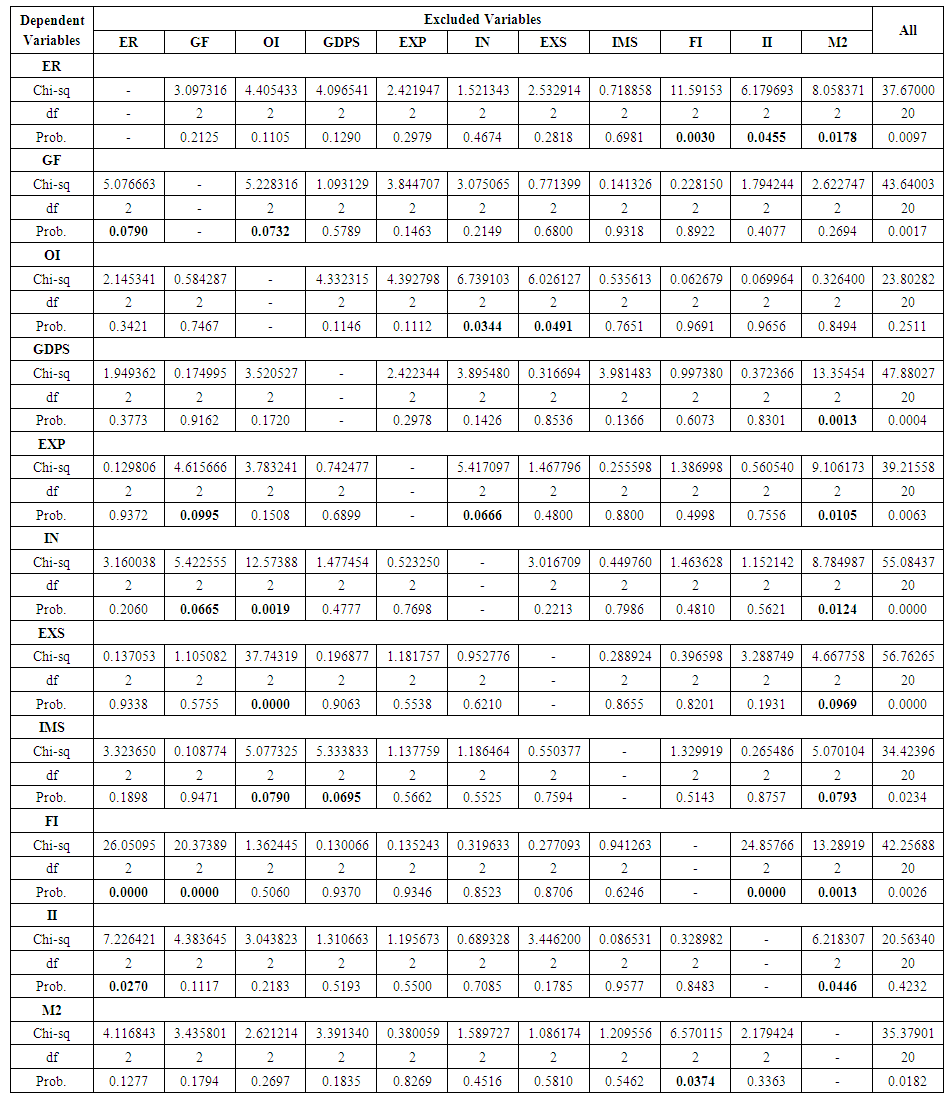 | Table (3). VAR Granger Causality/Block Exogeneity Wald Tests |
Table (4). Roots of Characteristic Polynomial for Exogenous variables C and Endogenous variables ER, GF, OI, GDPS, EXP, IN, EXS, IMS, FI, II and M2 with Lag specification: 1 2
 |
| |
|
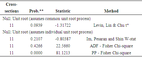
Table (5). Group unit root test: Summary for Series: ER, EXP, EXS, FI, GDPS, GF, II, IMS, IN, M2 and OI with lag length selection based on SIC from 0 to 13
 |
| |
|
4. Principal Component Analysis
For the purpose of policy-making and prioritization for economy of Iraq, principal component analysis is used. By using Kaiser criterion, we have three eigenvalues greater than one 6.084415, 2.18072 and 1.210415, so we have three factors. These factors contain 86.13% of information. The corresponding information for each factor taken as a percentage (86.13% will be treat as total information; by meaning that without losing a significant part of the original information) is as follows respectively, 64.2%, 23% and 12.8%.The factors are,(1) The first factor contains; Exchange Rate in market price (ER) variable (with a percentage of 17.2% (based on the information contained in the factor only) and 11% (based on all information included in the analysis), Exports (EX) variable (with a percentage of 20% (based on the information contained in the factor only) and 12.8% (based on all information included in the analysis), Gross Foreign Assets of CBI (GF) variable (with a percentage of 21.6% (based on the information contained in the factor only) and 13.9% (based on all information included in the analysis), Imports (IM) variable (with a percentage of 20.9% (based on the information contained in the factor only) and 13.5% (based on all information included in the analysis) and Broad Money (M2) variable (with a percentage of 20.3% (based on the information contained in the factor only) and 13% (based on all information included in the analysis).(2) The second factor contains; Foreign Investment (FI) variable (with a percentage of 28.4% (based on the information contained in the factor only) and 6.6% (based on all information included in the analysis), Gross Domestic Product In Constant Price (2007=100) (GDP) variable (with a percentage of 18.2% (based on the information contained in the factor only) and 4.2% (based on all information included in the analysis), Iraqi Investment (II) variable (with a percentage of 28.9% (based on the information contained in the factor only) and 6.6% (based on all information included in the analysis) and Oil price (OI) variable (with a percentage of 24.5% (based on the information contained in the factor only) and 5.6% (based on all information included in the analysis).(3) The third factor contains; Expenses (EXP) variable (with a percentage of 53.3% (based on the information contained in the factor only) and 6.8% (based on all information included in the analysis) and Income (IN) variable (with a percentage of 46.7% (based on the information contained in the factor only) and 6% (based on all information included in the analysis).Based on the above results, all plans, policies and programs of economic and development in Iraq must be made according to the effects of factors and consequently variables under consideration.
5. Summary
Most important eleven variables in Iraqi economy have been considered. Some of these variables have been compiled on an annual basis, while the other variables were compiled on a monthly basis. To unify these basis, the monthly values of these variables are simulated. VAR model is estimated and all related tests and indicators are obtained. The VAR model presented here has become ready for Iraqi economy explanation and forecasting. principal component analysis is used for the purpose of policy-making and prioritization for economy of Iraq. According to the effects of factors and consequently variables under consideration, plans and policies of economic and development in Iraq must be done.
ACKNOWLEDGMENTS
The author would like to thank Mr. Ali M. Al-Alaq, the governor of the central bank of Iraq and Dr. Mahdi M. Al-Alaq, the secretary – general of the council of Iraqi ministers for their continued support.
Appendix
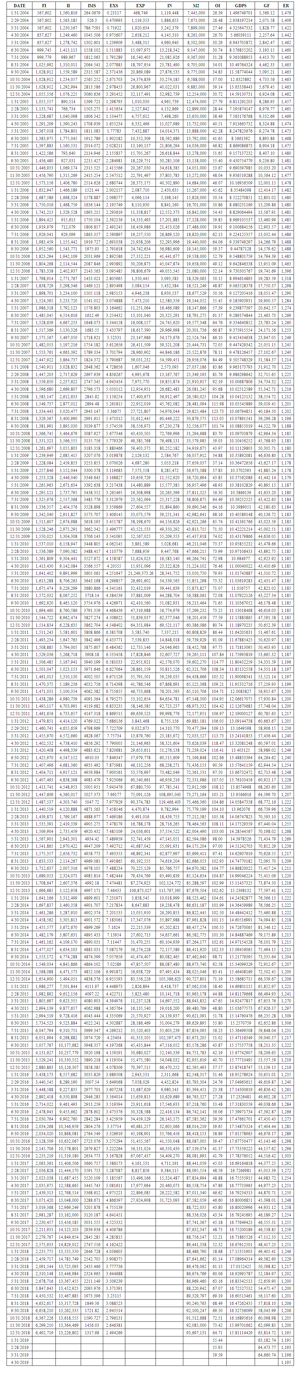 | Table (1). Data of variables under consideration, Foreign Investment (FI), Iraqi Investment (II), Imports (IM), Exports (EX), Expenses (EXP), Income (IN), Broad Money (M2), Oil price (OI), Gross Domestic Product In Constant Price (2007=100) (GDP), Gross Foreign Assets of CBI (GF) and Exchange Rate in market price (ER) |
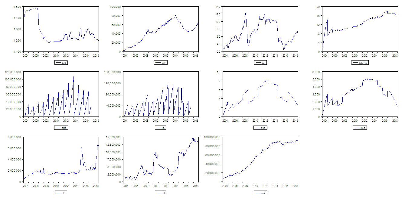 | Figure (1). Graphs of Series of Variables under consideration |
References
| [1] | Aikman, D. (2019) “Discussion of: ‘Forecasting and stress testing with quantile vector autoregression’ by Sulkhan Chavleishvili and Simone Manganelli”, Deutsche Bundesbank Spring Conference 2019: Systemic Risk and the Macroeconomy, Bank of England. |
| [2] | Akaike, H. (1973) “Information theory and an extension of the maximum likelihood principle”, In: Petrov B, Csáki F (eds) 2nd International Symposium on Information Theory, Académiai Kiadó, Budapest, pp 267–281. |
| [3] | Athanasopoulos, G., Guillén, O., Issler, J. and Vahid, F. (2010) “Model selection, estimation and forecasting in VAR models with short-run and long-run restrictions”, Working paper 205, central bank of Brazil. |
| [4] | Demeshko, M., Washio, T., Kawahara, Y. and Pepyolyshev, Y. (2016) “A Novel Continuous and Structural VAR Modeling Approach and Its Application to Reactor Noise Analysis”, ACM Transactions on Intelligent Systems and Technology (TIST), Vol. 7, Issue 2, pp.1-22. |
| [5] | Emmanuel, A. (2015) “Modeling GDP using VAR models: An empirical evidence from Ghana”, Master thesis, School of graduate studies, University of Ghana. |
| [6] | Forni, M, Gambetti, L. and Sala, L. (2018) “Structural VARs and noninvertible macroeconomic models”, Journal of applied econometrics, Vol. 34, Issue 2, pp. 221-246. |
| [7] | Gudeta, D., Arero, B. and Goshu, A. (2017) “Vector Autoregressive Modelling of Some Economic Growth Indicators of Ethiopia”, American Journal of Economics, Vol.7, Issue. 1, pp. 46-62. |
| [8] | Hamilton, J. (1994) “Time series analysis”, Princeton university press, new Jersey, USA. |
| [9] | Granger, J. (1969) “Investigating causal relations by econometric models and cross-spectral methods”, Econometrica 37, pp.424-438. |
| [10] | Hannan, E. and Quinn, B. (1979) “The determination of the order of an autoregression”, Journal of the royal statistical society, series B, Vol.41, pp. 190-195. |
| [11] | Hecq, A., Margaritella, L. and Smeekes, S. (2019) “Granger Causality Testing in High-Dimensional VARs: a Post-Double-Selection Procedure”, School of Business and Economics, Maastricht University, arXiv:1902.10991v1. |
| [12] | Huber, F. and Pfarrhofer, M. (2019) “Dealing with cross-country heterogeneity in panel VARs using finite mixture models”, University of Salzburg, Salzburg Centre of European Union Studies. arXiv:1804.01554v2. |
| [13] | Johansen, S. (1995) “Likelihood-based inference in cointegrated vector autoregressive models”, Oxford University Press, Oxford. |
| [14] | Kononenko, R. (2015) “IMF Lending and Economic Growth: An Empirical Analysis of Ukraine”, MSc thesis, College of Human Ecology, Cornell University, Ithaca, NY, USA. |
| [15] | Lütkepohl, H. (2005) “New Introduction to Multiple Time Series Analysis”, Springer, New York, USA. |
| [16] | Sims, C. (1980) “Macroeconomics and reality”, Econometrica, Vol.48, Issue 1, pp.1-48. |
| [17] | Sims, C. and Zha, T. (2006) “Does monetary policy generate recessions?”, Macroeconomic Dynamics, Vol.10, Issue 2, pp.231–272. |
| [18] | Warsono, E., Wamiliana, W. and Usman, M. (2019) “Vector Autoregressive with Exogenous Variable Model and its Application in Modeling and Forecasting Energy Data: Case Study of PTBA and HRUM Energy”, International Journal of Energy Economics and Policy, Vol. 9, Issue 2, pp.390-398. |

 Abstract
 Reference
 Full-Text PDF
 Full-text HTML