G. Ogwang1, D. N. Kamuganga2, T. Odongo3
1Faculty of Business and Management Sciences, Mbarara University of Science and Technology, Mbarara, Uganda
2Department of Philosophy and Development Studies, Makerere University, Kampala, Uganda
3Department of Economics, Makerere University Business School, Kampala, Uganda
Correspondence to: G. Ogwang, Faculty of Business and Management Sciences, Mbarara University of Science and Technology, Mbarara, Uganda.
| Email: |  |
Copyright © 2019 The Author(s). Published by Scientific & Academic Publishing.
This work is licensed under the Creative Commons Attribution International License (CC BY).
http://creativecommons.org/licenses/by/4.0/

Abstract
This study investigates the determinants of oil imports for Uganda in the period between 1993 and 2016 using VECM. The results in this study discovered that world oil price, Gross Domestic Product (GDP), changes in real relative prices (REER) and household final consumption expenditure determine oil import for Uganda both in the short and the long run but by statistically insignificant amount. Nevertheless, although the determinants of oil import to Uganda may be statistically insignificant both in the short and the long run, oil is an essential commodity in Uganda such that any increase or decrease in the factors determining oil imports into Uganda cannot discourage oil import into the country. The policy implication for this study is that world oil price, REER and household final consumption expenditure may not be the only variables that determine oil import for Uganda both in the short and the long run, there are therefore a combination of other factors operating in the economy that may determine oil import for Uganda.
Keywords:
Determinants of Oil Imports, Vector Error Correction Model (VECM), Real Effective Exchange Rate (REER), Household Final Consumption Expenditure (HHE), World Crude Oil Price (WOP)
Cite this paper: G. Ogwang, D. N. Kamuganga, T. Odongo, Understanding the Determinants of Uganda’s Oil Imports, American Journal of Economics, Vol. 9 No. 4, 2019, pp. 181-190. doi: 10.5923/j.economics.20190904.03.
1. Introduction
The relationship between oil price shocks and economic activity has become a center of interest to many researchers around the world and the recent decline of oil prices has even amplified the interest of many scholars in this area (Suleiman, 2013; Baffes, Kose, Ohnsorge and Stocker, 2015).Theoretically, for oil-importing developing economies like Uganda, the decline in oil prices should support stronger growth, reduce inflation, and improve external and fiscal balances, which should lower macroeconomic vulnerabilities and, therefore, widen policy room. Fuel price shocks could result into indirect effects such as food prices (through transport and production input costs) as well as on economic activity more broadly, ultimately affecting jobs, livelihoods, and then household income (Mendoza, 2009). In addition, households use a variety of petroleum products: kerosene for lighting, cooking, and heating water; liquefied petroleum gas (LPG) for cooking and heating; and gasoline and diesel for private vehicles as well as thermal power generation.Higher oil prices, on the other hand, lower effective household income in three ways. First, households pay more for petroleum products they consume directly. Secondly, higher oil prices increase the prices of all other goods that have oil as an intermediate input. For the poor who use transport services, higher transport costs also decrease effective income. To some extent, higher oil prices could lower GDP growth and household income in developing countries (Kojima, Matthews and Sexsmith, 2010).Crude oil and its constituent products such as diesel, petrol/gasoline, liquefied petroleum gas (LPG), kerosene among others are major drivers of businesses, manufacturing, transportation of goods and services in Uganda, regional and global level.Uganda has neither crude oil production nor a refinery and is totally dependent on imports of petroleum products, although it has recently discovered some oil reserves in the country. About 90 percent of Uganda’s petroleum imports are routed through Kenya with only 10 percent coming through Tanzania. There are many licensed oil-marketing companies in Uganda with Shell and Total dominating the downstream market countrywide. The performance of world oil prices, the value of oil imports into Uganda as well as domestic petrol/gasoline prices in the period between 1993 and 2016 has been shown in figure 1, 2, 3 and 4.As shown in figure 1 and 2 below, there is a general trend in the increase of world oil prices while the value of oil imports in Uganda is strangely increasing during this period. Further, the behaviour of the value of oil imports and the performance of domestic prices have been surprising. The value of imports has been increasing while the general trend of domestic pump price for oil has also been increasing as shown in figure 2, 3 and 4.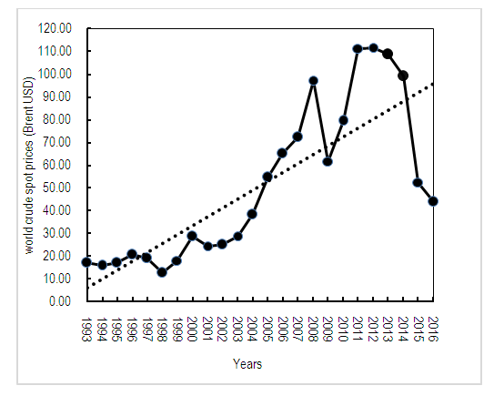 | Figure 1. World spot crude oil prices (Source: Author’s analysis) |
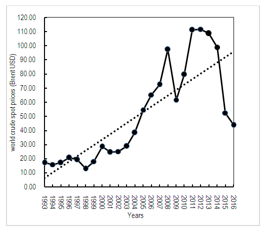 | Figure 2. Trend in Value of Oil Import into Uganda (Source: Author’s analysis) |
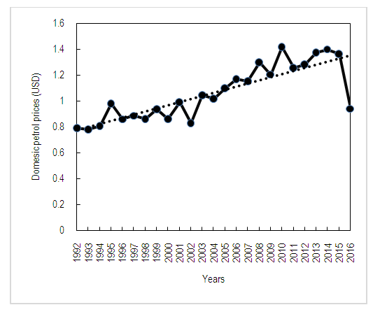 | Figure 3. Trend of Domestic Petrol Prices (Source: Authors analysis) |
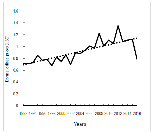 | Figure 4. Trend of Domestic Diesel Prices (Source: Authors analysis) |
The above performance may lead to a conclusion that performance of oil import during this period does not in any way affect domestic oil prices. The increase in pump prices in the period following the increase in the value of oil import is the cause of concern and points to the possible effect of other factors than oil import to be shaping Uganda’s domestic oil pump prices and is the cause for this study.
2. Empirical Background
The theoretical underpinning for the determinants of oil imports arises from the standard framework of modelling energy demand which is derived from the Marshallian (Marshall, 1890) demand theory for goods and services. A Marshallian demand curve reflects both substitution and income effects. Movements along it show how the quantity demanded changes as price changes (holding all other prices and income constant), so it reflects both the substitution and the income effects. Marshall acknowledged that, owing to joy and excitement, the rate of expenditure incurred by a consumer over a certain period may well surpass the rate that his ability permits. Afterwards, the consumer should become aware of this possibility and should learn to control his expenditure (Biswa, 2012). Marshall demand function is part of the consumer theories. Consumer theory is concerned with how a rational consumer would make consumption decisions. It emphasizes consumption or demand for goods and services by utility-maximizing individuals. Utility-maximizing individuals make choices that maximize the satisfaction received from present and future consumption. According to a study by Yaprakli and Kaplan (2015) that examined the Turkish crude oil import demand for the period of 1970-2013, their empirical results show that income and price elasticities of demand for crude oil import in the long-run are inelastic.Asuamah and Ohene-Manu (2015) examined the long run and short-run determinants of fossil fuel consumption in Ghana for 1970-2011 period by using Autoregressive distributed lag model (ARDL). The results suggested that macroeconomic variables such as income, price, trade openness, investment, money supply, and government expenditure do not play an observable role in fossil fuel consumption hence they could not be relied on as a policy tool to manage fossil fuel consumption.The results of the study on determinants of oil imports in Ghana by Marbuah (2017) show that demand for crude oil is price inelastic in the short-run but elastic in the long-run. Other important drivers of crude oil import are the real effective exchange rate, domestic oil production and population growth. Income is found to be the strongest driver of crude oil demand (Marbuah, 2017).A study on China by Xiong and Xu (2009) recognized oil, GDP, population growth and share of the industrial sector in GDP as the drivers of crude oil demand. Zhao and Wu (2007) study the factors that determine oil imports into China by considering the price of crude oil, domestic energy production (including crude oil), industrial output and total traffic volume as potential determinants. The above study finds a significant, positive and inelastic price elasticity relationship with oil imports.Tsirimokos (2011) evaluated price and income elasticities for crude oil demand in Sweden, Denmark, Spain, Portugal, Turkey, Finland, Italy, Germany, USA and Japan. With Nerlove's partial adjustment model, the results show both price and income elasticities are more inelastic in the short-run than in the long-run.Narayan and Smyth (2007) study on 12 Middle East countries finds that the income elasticity variable differs across countries but at the panel level, consumers are insensitive to price changes. They find that the demand for oil in the Middle East is significantly driven by income.Iwayemi, Adenikinju and Babatunde (2010) demonstrate that petroleum products are both price and income inelastic in Nigeria. Jabir (2009) study showed that the U.S GDP plays a leading role together with domestic oil production in determining oil imports.As seen from above, the determinant of oil imports is not clear cut as one move from one country to another, being developed and developing countries, oil importing and oil exporting nations. In particular, there are no know studies on the determinants of oil imports into Uganda and yet oil is an important driver of Ugandan economy.
3. The Data and Model
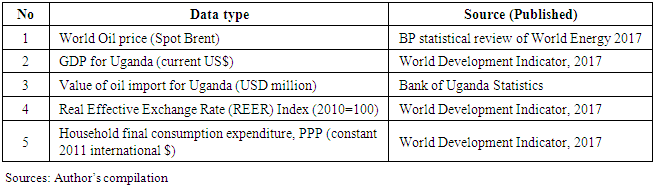
The data type in this study are secondary from 1993 to 2016. The details of the data types and sources in this study are presented in table 1 below.Table 1. Data Type and Sources
 |
| |
|
3.1. Description of Data Set
The details of the data used in the study are presented below.
3.1.1. World Crude Oil Price
The study used spot price Brent as a proxy to world crude oil prices since is the most applicable to the study as it is widely used as a benchmark for crude oil pricing. According to EIA (2014), the most widely used benchmarks are associated with crude oil that has four common qualities: stable and ample production; a transparent, free-flowing market located in a geopolitically and financially stable region to encourage market interactions; adequate storage to encourage market development; and/or delivery points at locations suitable for trade with other market hubs, enabling arbitrage (profit opportunities) so that prices reflect global supply and demand. It has been assumed in the study that, the higher world oil price would result into a lower value of oil imported during the period under consideration. The data for Brent spot price was obtained from BP statistical review of World Energy 2017.
3.1.2. Value of Oil Import for Uganda (USD million)
This capture the value of oil imported in Uganda in USD million from 1993 to 2016. The quarterly data were obtained from the Bank of Uganda Statistics, 2017. It has been assumed in the study that value of oil imports in Uganda is affected by world crude oil price, with higher world prices resulting into reduced value of oil imports.
3.1.3. Gross Domestic Product (GDP)
This captures the nature of economic activity in Uganda. It has been assumed that the higher the real GDP, the higher is the demand for oil imports. Higher domestic oil/fuel pump prices negatively affect the level of economic activity. The annual GDP (current USD) data were obtained from the World Development Indicator, 2017.
3.1.4. Real Effective Exchange Rate (REER)
The inclusion of real effective exchange rate (REER) in the model was vital since oil price on the world market is quoted in US dollars. Real effective exchange rate is the nominal effective exchange rate (a measure of the value of a currency against a weighted average of several foreign currencies) divided by a price deflator or index of costs. In addition, any change in the exchange rate of the local currency against the USD affect the domestic price of oil and the real value of wealth and thus the demand for oil. Since Uganda is generally a net importer of crude oil and a price-taker, any changes in the exchange rate will influence demand for crude. An increase in REER implies that exports become more expensive and imports become cheaper and hence an increase indicates a loss in trade competitiveness. The quarterly data of Real Effective Exchange Rate (REER) Index (2010=100) were obtained from the World Development Indicator, 2017.
3.1.5. Household Final Consumption Expenditure
Household final consumption expenditure, Purchasing Power Parity (PPP) (constant 2011 international USD) is expected to increase national energy consumption through per capita consumption in key areas such as transportation. PPP conversion factor is the number of units of a country’s currency required to buy the same amounts of goods and services in the domestic market as U.S. dollar would buy in the United States. This conversion factor is for private consumption (i.e. household final consumption expenditure). The data were obtained from the World Development Indicator 2017 of the World Bank.
3.2. Model Specification
This study uses VECM to investigate the determinants of oil imports for Uganda. The details of which are indicated below.Following Bruce and Natalie (2003), the general form of VECM is as follows; | (1) |
Where Xt is an nx1 matrix and n-vectors of dependent variables,  and
and  are parameters, while Vt is a residual. An error correction mechanism is evidenced in the Error Correction Term (ECTt-1). There are many error correction terms as there are co-integrating vectors (r). Parameter
  associated with Error Correction Term (ECTt-1) measures proportion of adjustment back towards an equilibrium that can be completed within a single period. If parameter
  is not significantly different from zero then there is no error correction process working within the model. Parameter
  , on the other hand, indicates the presence of a short term lag from one variable to another and it measures short term adjustment back towards equilibrium (Odongo, 2013). The study used the variables in Marbuah (2017) who investigated oil import demand in Ghana. Following from the standard framework of modelling energy demand which is derived from the Marshallian demand theory for goods and services, the study formulated basic crude oil import demand model, consistent with the literature, as a function of real income and the international price of crude oil. The study also included other two variables (Household final consumption expenditure and Real Effective Exchange Rate) which were equally important. The model for this study is as in (2) and (3);
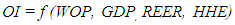 | (2) |
Equation (4) is expressed in logarithmic form as follows: | (3) |
Where;OI = Value of crude oil import for Uganda in US$ millionGDP = Gross Domestic Product of Uganda (Current USD)WOP= World crude oil price (proxy to spot Brent in US Dollars per Barrel).REER= Real effective exchange rateHHE= Household final consumption expenditureμ= Error term assumed to satisfy all the residual regression assumptions of no serial correlation, homoscedasticity and normality.α0, α1, α2, α3, α4 > 0This is the model (equation 3) for the determinants of oil imports in Uganda. The model assumes that oil imports increase with a fall in world oil prices, an increase in the GDP, an appreciation in REER and an increase in household final consumption expenditure for Uganda.
3.3. Data Estimation Techniques
This section explains he techniques for data analysis, details of which are indicated below.
3.3.1. Stationary Test
The stationarity test in this study used regressions of time series data analyzed against a constant. These regressions were expressed as follows; 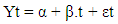 | (4) |
 | (5) |
The stationarity of residuals  were tested. The series were examined for stationarity using Philips Perron (PP) test and Kwiatkowski, Phillips, Schmidt and Shin (KPSS) test using a lag selected by Schwarz Information Criterion (SIC). The first step in determining stationarity involved graphing the data to observe its behaviour. The next step involved conducting a unit root test. The null hypothesis of PP is that the series has a unit root (non-stationary) and rejecting the null hypothesis of the PP unit root test implies the series is stationary. The null hypothesis of the KPSS test is that the series stationary and rejecting the null hypothesis of the KPSS stationarity test implies the series is non- stationary. KPSS test for stationary around a deterministic trend (i.e. trend-stationary).
3.3.2. Cointegration Test
The necessary criteria for stationarity among non-stationary variables is called cointegration. Testing for cointegration is necessary step to check if one is modelling empirically meaningful relationships. For this study, Johnsen test procedure was adopted to test for cointegrating relationship within endogenous variables based on Maximum Likelihood (LM) test and unrestricted Vector Auto Regression (VAR) test. Cointegration rank r (number of cointegrating vectors) was tested using trace statistics and Maximum Eigen Statistics (MES).
3.3.3. Vector Error Correction Model (VECM)
A vector error correction (VECM) model is a restricted VAR designed for use with non-stationary series that are known to be cointegrated. The VECM has co-integration relations built into the specification so that it restricts the long-run behaviour of the endogenous variables to converge to their cointegrating relationships while allowing for short-run adjustment dynamics. The co-integration term is known as the error correction term since the deviation from long-run equilibrium is corrected gradually through a series of partial short-run adjustment (E-views, 2017). VECM has been used to determine whether there exists any short run or long run causal relationship within the variables in the model specified. The presence of co-integrating relationship within endogenous variables is a necessary condition for estimating vector error correction model. VECM specification only applies to cointegrated series, hence one should first run the Johansen cointegration test and determine the number of cointegrating relations. Generally, the stationary and cointegration of data must be checked before using VECM. In testing the stationary data, a combination of time series plot and unit root test using both Philips Perron (PP) and Kwiatkowski, Phillips, Schmidt and Shin (KPSS) test was used. The next step was to test for the cointegration using Johansen cointegration test method to determine the long term relationship among the variables used in this study. After confirming the presence of co-integration between the variables, and that the variables are integrated of order one in the stationary test, the study then proceeded with the estimating of the Vector Error Correction Model (VECM) using E-views. In estimating the VECM, the optimum lag has been determined by comparing every lag to the criteria used (Schwarz Information Criterion) and choosing the minimum values from the information criteria. After selection of the lag length, the VECM was estimated, diagnosed and interpreted.One of the advantages of VECM is that VAR model can suggest only a short-run relationship between the variables since the long-run information is removed by first differencing, while the ECM avoids this. Furthermore, the ECM distinguishes between a long- and short-run relationship and can identify causation sources that cannot be detected by the usual causality test. The challenge with VECM, according to Gonzalo (1994) is that underspecifying the number of lags in a VECM could lead to serial correlation and increase the finite-sample bias in the parameter estimates.
4. Presentation and Discussion of the Results
The results of this study are obtained from the estimates of VECM. Details of the results are presented below. The non-normality could have been caused by excess kurtosis. The study proceeds with stationarity test on the variables using unit root test.
4.1. Descriptive Statistics
The summary statistics in table 2 below indicate that normality test has been rejected in all the 5 variables at 5 percent level of significance. Table 2. Descriptive Statistics
 |
| |
|
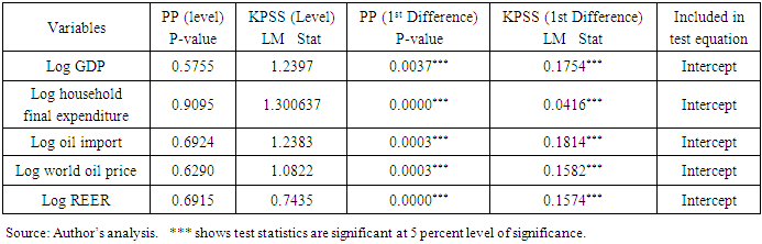
4.2. Test for Stationarity
The stationarity test has been carried out using Philips Perron (PP) and Kwiatkowski, Phillips, Schmidt and Shin (KPSS) test. The null hypothesis of PP test is that the series has a unit root and if the computed p-value is less than the significance level (1 percent, 5 percent and 10 percent), then one rejects the null hypothesis at those respective levels of significance. However, the null hypothesis of KPSS test is that the series is stationary and if the computed LM statistics is more than that of the critical values at significance level (1 percent, 5 percent and 10 percent), then one rejects the null hypothesis. The summary of the stationarity test is presented in table 3.Table 3. Stationary Test for Variables under Study
 |
| |
|
The results in table 3 show that using PP and KPSS tests, all other variables are non-stationary at levels at 5 percent level of significance. In their first difference, all the variables are stationary at 5 percent level of significance. The study proceeds to test for cointegration among the variables under study.
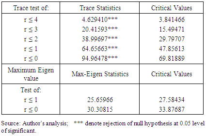
4.3. Test for Cointegration
Cointegration test has been carried out in this study to determine if there exists any long-run relationship within variables in the model specified. The results for the Johansen cointegration test carried out in the study are presented in table 4 below.Table 4. Cointegration Test Results
 |
| |
|
The results from Unrestricted Trace Statistics (UTS) in this table indicate five cointegrating vectors at 0.05 percent level of significance; while the results from Maximum Eigen Statistics (MES) in the same table also indicate no co-integrating vectors at 0.05 percent level of significance. Thus; there exists a long run relationship within variables in the model specified which is a necessary condition for running VECM.
4.4. Diagnostic Test
Following the cointegration test carried out in this study, the study proceeds to carry out the normality test in order to determine whether the data series in this study are normally distributed or not. Further, Autoregressive Conditional Heteroskedasticity (ARCH) test has been carried out in this study to determine whether there exists serial correlation in the variables specified in the study and finally, the study carried out Regression Specification Error Test (RESET) to determine whether there exists misspecification error among the variables specified in the study. Details of the diagnostic test carried out in this study are indicated below.
4.4.1. Normality Test
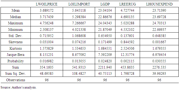
Normality test has been carried out in this study to determine whether the data series estimated in the study are normally distributed or not. The result in figure 5 displays a histogram and descriptive statistics of the residuals, including the Jarque-Bera statistic that tests for normality. If the residuals are normally distributed, the histogram should be bell-shaped and the Jarque-Bera statistic should not be significant. The reported probability in the above table, indicates that the Jarque-Bera statistic probability is significant (4.7 percent). This study therefore concludes that there is non- normal distribution among the data series.Following the normality test, this study proceeds to test for serial correlation using Autoregressive Conditional Heteroskedasticity (ARCH) test. Details of the ARCH test carried out in this study are indicated below.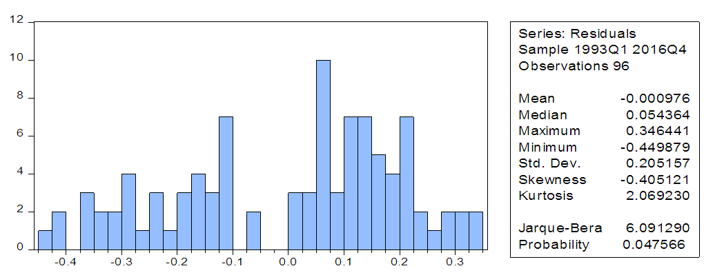 | Figure 5. Normality Test Results (Source: Author’s analysis) |
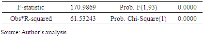
4.4.2. Autoregressive Conditional Heteroskedasticity (ARCH) Test
The ARCH test uses autocorrelations and partial autocorrelations of the squared residuals to determine whether there exists any serial correlation in the residual of the variables in the model specified. Details of the results from the ARCH test carried out in this study are presented in table 5. Table 5. Heteroskedasticity Test: ARCH
 |
| |
|
A small p-value (typically ≤ 0.05) indicates strong evidence against the null hypothesis, meaning rejecting the null hypothesis. Under the null hypothesis of no ARCH up to order 1 in the residuals, the probability of rejecting Ho is 0.00. At 1 percent level of significance, this study, therefore, reject the null hypothesis of no ARCH in the variables in this study.
4.4.3. Regression Specification Error Test (RESET) for Misspecification
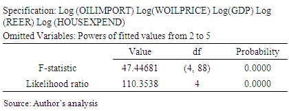
Regression Specification Error Test (RESET) has been carried out in this study to test for specification error in the variables specified in the study. Details of the results from the RESET test in this study are indicated in table 6 below. Table 6. Ramsey RESET Test
 |
| |
|
The RESET F-statistic has a p-value of 0.00 percent and Likelihood ratio has a p-value of 0.00 percent, indicating that the null hypothesis has been rejected at 1 percent level of significant. A small p-value (typically ≤ 0.05) indicates strong evidence against the null hypothesis, meaning rejecting the null hypothesis. Following the diagnostic tests, the study proceeds to estimate the determinants of Uganda’s oil imports in the period under the review using VECM.
4.5. Vector Error Correction Model (VECM)
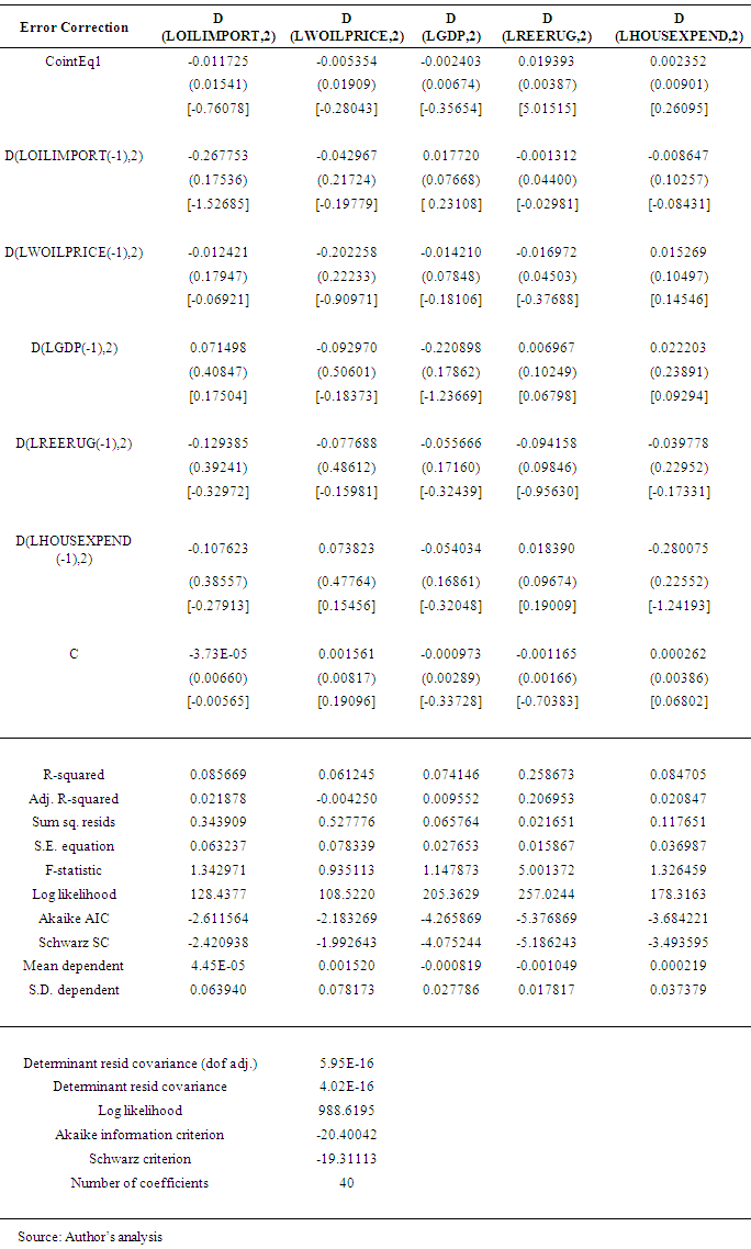
Vector Error Correction Model (VECM) has been used to determine whether there exists any short run or long run causal relationship within the variables in the model specified. The presence of co-integrating relationship within endogenous variables is a necessary condition for estimating vector error correction model and it shows that there exists long-run error correction mechanism working within the model such that any deviation from the long run equilibrium would be restored by correction of equilibrium error towards its long-run relationship. The co-integration test showed the presence of co-integration in the model specified, hence validating the use of VECM. The results of the VECM is presented in table 7 below. The results shown in the table 7 gives the estimated parameters in each of the five forms of VECM equations which are drawn from each column. Row number one gives the Error correction term (ECT) for each of the equation. The estimated parameters on ECT are presented in the row number one and their standard errors are in row number two, while t ratios are presented in row number three. The results of the long run relationship in table 7 below show that a 1 percent increase in world oil price reduces the oil imports by 0.005 percent, 1 percent increase in GDP decreases the oil imports by 0.002 percent, 1 percent increase in real effective exchange rate (REER) increases oil imports by 0.02 percent, and 1 percent increase in household final consumption expenditure increases the oil imports by 0.002 percent. Thus, the result for the long run relationship in this study can be summarized as in the equation (6) below. | (6) |
Table 7. VECM Results
 |
| |
|
Although the effect of these variables are statistically insignificant in the long run, it can be said that the effect of world oil price, domestic income (GDP), changes in relative prices (REER) and household final consumption expenditure determines oil import for Uganda but in insignificant amount. It can also be realized that oil is an essential commodity in Uganda such that increase or decrease in its world price and also increase or decrease in domestic income (GDP) do not significantly affect its import. Secondly, it can also be realized that appreciation or depreciation in relative prices (REER) as well as increase or decrease in household final consumption expenditure on other goods and services do not discourage oil import to Uganda in the long run.The results for the short term relationship in the VECM in table 7 above indicate that 1 percent increase in world oil price decreases the oil imports by 0.01 percent, 1 percent increase in GDP increases oil imports by 0.07 percent, 1 percent increase in real effective exchange rate (REER) decreases oil imports by 0.13 percent, and 1 percent increase in household final consumption expenditure decreases the oil imports by 0.11 percent. Thus, the result for the short run relationship in this study be summarized as in the equation (7) below. | (7) |
Although the effect of the above variables are statistically insignificant, it can be said that the effect of world oil price, domestic income (GDP), changes in relative prices (REER) and household final consumption expenditure determines oil import for Uganda but in insignificant amount in the short run. It can also be realized that oil is an essential commodity in Uganda such that increase or decrease in its world price and also increase or decrease in domestic income (GDP) do not significantly affect its import. Secondly, it can also be realized that appreciation or depreciation in relative prices (REER) as well as increase or decrease in household final consumption expenditure on other goods and services do not discourage oil import in the short run.
5. Conclusions
This study investigates the determinants of oil imports for Uganda in the period between 1993 and 2016 using VECM. The results in this study discovered that world oil price, Gross Domestic Product (GDP), changes in real relative prices (REER) and household final consumption expenditure determine oil import for Uganda both in the short and the long run but by statistically insignificant amount. Nevertheless, although the determinants of oil import to Uganda may be statistically insignificant both in the short and the long run, oil is an essential commodity in Uganda such that any increase or decrease in the factors determining oil imports into Uganda cannot discourage oil import into the country.
6. Policy Implications
The policy implication for this study is that world oil price, REER and household final consumption expenditure may not be the only variables that determine oil import for Uganda both in the short and the long run, there are therefore a combination of other factors operating in the economy that may determine oil import for Uganda.
References
| [1] | Asuamah, S. Y., & Ohene-Manu, J. (2015). An Econometric Investigation of the Determinants of Fossil Fuel Consumption: A Multivariate Approach for Ghana. Economy, 2(1), 32–43. |
| [2] | Baffes, J., Kose, M. A., Ohnsorge, F., & Stocker, M. (2015). The Great Plunge in Oil Prices: Causes, Consequences , and Policy Responses. The World Bank. |
| [3] | Biswa, T. (2012). The Marshallian Consumer. Review of Economic Analysis, 4, 165–174. |
| [4] | Bruce, F., & Natalie, J. (2003). Population Change and Australia Living Standard (ISSN 1443-8593). Retrieved from www.utas.edu.au/economics. |
| [5] | E-views. (2017). User’s Guide: Multiple Equation Analysis: Vector Autoregression and Error Correction Models: Vector Error Correction (VEC) Models. Retrieved from https://0x9.me/Ej2cz. |
| [6] | EIA. (2014). Benchmarks play an important role in pricing crude oil. Retrieved from from https://www.eia.gov/todayinenergy/detail.php?id=18571. |
| [7] | Gonzalo, J (1994). Five alternative methods of estimating long-run equilibrium relationships. Journal of Econometrics, 60, 1-2, 203-233. |
| [8] | Iwayemi, A., Adenikinju, A., & Babatunde, M.A., (2010). Estimating petroleum products demand elasticities in Nigeria: a multivariate cointegration approach. Energy Economics 32, 73-85. |
| [9] | Jabir, I., (2009). The dynamic relationship between the US GDP, imports and domestic production of crude oil. Appl. Econ. 41 (24), 3171–3178. |
| [10] | Kojima, M., Matthews, W. & Sexsmith, F. (2010). Petroleum markets in Sub-Saharan Africa: analysis and assessment of 12 countries (English). (World Bank, Extractive industries and development series No. 15). Retrieved from http://documents.worldbank.org/curated/en/907171467990361424/Petroleum-markets-in -Sub-Saharan-Africa-analysis-and-assessment-of-12-countries. |
| [11] | Marbuah, G. (2017). Understanding crude oil import demand behaviour in Africa: The Ghana case. Journal of African Trade, 4(1–2), 75–87. https://doi.org/10.1016/j.joat.2017.11.002. |
| [12] | Marshall, (1890). Principles of Economics, London: Macmillan. |
| [13] | Mendoza, R. U. (2009). Aggregate Shocks, Poor Households and Children: Transmission Channels and Policy Responses. Global Social Policy, 9(1 Suppl), 55–78. |
| [14] | Narayan, P.K., & Smyth, R. (2007). A panel cointegration analysis of the demand for oil in the Middle East. Energy Policy 35, 6258-6265. |
| [15] | Odongo, T. (2013). The effect of trade liberation on Uganda’s lint export (PhD thesis, Makerere University). |
| [16] | Suleiman, M. (2013). Oil Demand, Oil Prices, Economic Growth and the Resource Curse: An Empirical Analysis (PhD thesis, University of Surrey). |
| [17] | Tsirimokos, C. (2011). Price and income elasticities of crude oil demand: The case of ten IEA countries (Master thesis, Department of Economics, Swedish University of Agricultural Sciences, Uppsala, Sweden). |
| [18] | Tweneboah, G., & Adam, A. M. (2008). Implications of Oil Price Shocks for Monetary Policy in Ghana: A Vector Error Correction Model. Munich Personal RePEc Archive(MPRA) Paper, (11968), 1–21. https://doi.org/10.2139/ssrn.1312366. |
| [19] | Yaprakli, S., & Kaplan, F. (2015). Re-examining of the Turkish crude oil import demand with multi-structural breaks analysis in the long run period. International Journal of Energy Economics and Policy, 5(2), 402–407. |
| [20] | Xiong, J., & Wu, P., (2009). An analysis of forecasting model of crude oil demand based on cointegration and vector error correction model (VEC). In 2008 International Seminar on Business and Information Management ISBIM 2008, 485-488. |
| [21] | Zhao, X., & Wu, Y. (2007). Determinants of China’s imports: an empirical analysis. Energy Policy 35, 4235-4246. |

 Abstract
 Reference
 Full-Text PDF
 Full-text HTML