1. Introduction

The relationship between oil price shocks and economic activity has become a center of interest to many researchers around the world and the recent decline of oil prices has even amplified the interest of many scholars in this area (Suleiman, 2013; Baffes, Kose, Ohnsorge and Stocker, 2015). It may seem that economists, policymakers, or financial market participants should be able to form accurate expectations about the future price of oil, if they actually understand the determinants of past oil price fluctuations, however, this is not necessarily the case. The reason is that the price of oil will only be as predictable as its determinants, even if economic models of the global oil market are approximately correct. Unless one can foresee the future evolution of these determinants, surprise changes in the price of oil driven by unexpected shifts in oil demand or oil supply will be inevitable (Baumeister & Kilian, 2016). Theoretically, oil price shocks should affect oil exporting and oil importing countries differently both at macroeconomic and microeconomic levels (Kilian, 2010; Mohaddes and Pesaran, 2016). For oil-importing developing economies like Uganda, the decline in oil prices should support stronger growth, reduce inflation and improve external and fiscal balances, which should lower macroeconomic vulnerabilities and, therefore, widen policy room. Fuel price shocks could result into indirect effects such as food prices (through transport and production input costs) as well as on economic activity more broadly, ultimately affecting jobs, livelihoods, and then household income (Mendoza, 2009).

Activity in oil importers should benefit from lower oil prices since a drop in oil prices raises household and corporate real incomes in a manner similar to a tax cut (Baffes et al., 2015).

Higher oil prices, on the other hand, lower effective household income in three ways. First, households pay more for petroleum products they consume directly. Secondly, higher oil prices increase the prices of all other goods that have oil as an intermediate input. For the poor who use transport services, higher transport costs also decrease effective income. To some extent, higher oil prices could lower GDP growth and household income in developing countries (Kojima, Matthews and Sexsmith, 2010).

Kilian (2014) pointed out that transmission of oil price shocks relies on two main channels. One immediate effect of an unexpected increase in the price of imported crude oil is a reduction in the purchasing power of domestic households, as income is being transferred abroad. The other immediate effect is to increase the cost of producing domestic output to the extent that oil is a factor of production along with capital and labour, which is akin to an adverse aggregate supply shock. These direct effects of an exogenous increase in the real price of oil imports are symmetric in oil price increases and decreases. An unexpected increase in the real price of oil will cause aggregate production and income to fall by as much as an unexpected decline in the real price of oil of the same magnitude will cause aggregate income and production to increase.

Balcilar, Eyden, Uwilingiye, and Gupta (2014), on the other hand, argue that there are a number of transmission channels through which oil price affects output of a country. On the supply side, an increase in the oil price leads to higher input costs which can increase the cost of production of goods and services. The volume produced may consequently be affected, as firms may find it not easy in the short run to reallocate resources in order to produce the matching volume of goods and services. The extent of the impact of oil price shocks to the aggregate output depends on the energy intensity in the production process. From the demand side, an increase in the oil price will put stress on the price level. In turn, the central bank might increase the interest rate to control inflation, which may result in a reduction in investment, and thus a decline in output. Besides, increase in oil price affects the individual consumer as it reduces the quantity of goods and services that may perhaps be purchased with the consumer's existing level of income (Balcilar et al., 2014).

Several factors, however, could counteract the global growth and inflation implications of the lower oil prices. These include weak global demand and limited scope for additional monetary policy easing in many countries. The disinflationary implications of falling oil prices may be muted by sharp adjustments in currencies and the effects of taxes, subsidies, and regulations on prices (Baffes et al., 2015).

Crude oil and its constituent products such as diesel, petrol/gasoline, liquefied petroleum gas (LPG), kerosene among others are major drivers of businesses, manufacturing, transportation of goods and services in Uganda, regional and global level.

Uganda has neither crude oil production nor a refinery and is totally dependent on imports of petroleum products, although it has recently discovered some oil reserves in the country.

The quest for higher economic growth rates imply need for adequate supply of crude oil and its constituent products for the domestic, industrial, agricultural and transport sectors of any economy. This therefore means that intervention in the energy sector and in particular oil subsector is very important for the economic development of Uganda.

The performance of world oil prices, the value of oil imports into Uganda as well as domestic pump prices in the period between 1993 and 2016 are presented in figure 1, 2, 3 and 4 (refer to section 3). As shown in figure 1 and 2, there is a general trend in the increase of world oil prices while the value of oil imports in Uganda is strangely increasing during this period. Further, the behavior of the value of oil imports and the performance of domestic prices have been surprising. The value of imports has been increasing while the general trend of domestic oil price has also been increasing as shown in figure 2, 3 and 4.

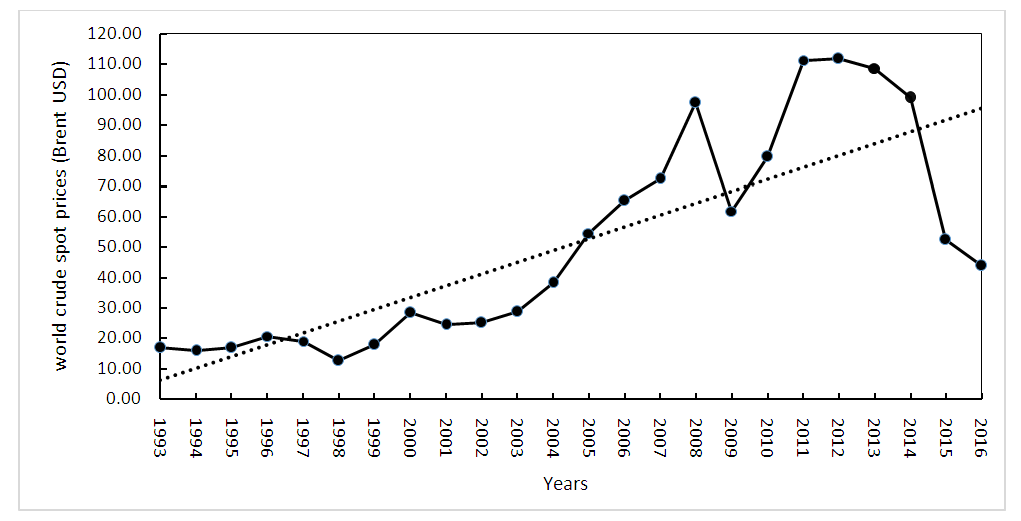Figure 1. World spot crude oil prices (1993 to 2016) (Source: Author’s analysis based on BP statistical review of World Energy 2017)

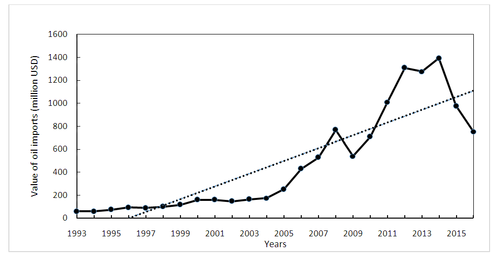Figure 2. Trend in Value of Oil Import into Uganda (1993 to 2016) (Source: Author’s analysis based on Bank of Uganda Statistics)

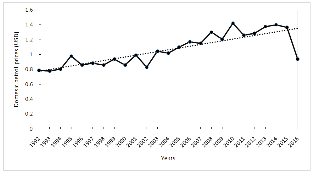Figure 3. Trend of Domestic Petrol Prices (1993 – 2016) (Source: Author’s analysis based on World Development Indicator, 2017)

Figure 4. Trend of Domestic Diesel Prices (1993 – 2016) (Source: Author’s analysis based on World Development Indicator, 2017)

Further to note, during the recent fall in global oil price period between the year 2014 and 2015 where the world oil price fell enormously by 47.06% (from 98.95 to 52.39 USD), domestic petrol price reduced by 2.5% (from 1.4 to 1.37USD) and domestic diesel pump prices increased by 1.08% (from 1.11 to 1.12USD). The case of strange nexus of behavior between the value of oil imports and domestic pump prices in relation to the changes in the world oil prices in the period under study is the cause of concern for this study.

2. Empirical Background

Oil price shocks and its transmission into national economies has been studied by many researchers using various econometrics methods including SVAR.

Kilian and Park (2009) conducted study on the impact of oil price shocks on the U.S. stock market using Structural VAR model. Their study showed that the reaction of U.S real stock returns to an oil price shock differs greatly depending on whether the change in the price of oil is driven by demand or supply shocks in the oil market. The demand and supply shocks driving the global crude oil market jointly account for 22% of the long-run variation in U.S. real stock returns. The responses of industry-specific U.S. stock returns to demand and supply shocks in the crude oil market are consistent with accounts of the transmission of oil price shocks that emphasize the reduction in domestic final demand.

Ghosh, Varvares, and Morley (2009) on the other hand conducted a study on the effects of oil price shocks on output of U.S using dynamic error correction model. Their preferred model suggests that oil prices reduced GDP growth by about 0.4 percentage point on average through the first three quarters of 2008, before contributing 1.7 percentage points in the fourth quarter as prices plummeted. Park and Ratti (2008) also studied the effect of oil price shocks on stock markets in the U.S. and 13 European countries using Vector autoregressive model (VAR). Their study showed that oil price shocks have a statistically significant impact on real stock returns contemporaneously and/or within the following month in the U.S. and 13 European countries over 1986:1–2005:12.

Norway as an oil exporter shows a statistically significantly positive response of real stock returns to an oil price increase. For many European countries, but not for the U.S., increased volatility of oil prices significantly depresses real stock returns. The contribution of oil price shocks to variability in real stock returns in the U.S. and most other countries is greater than that of interest rate.

Tang, Wu, and Zhang (2010) on the other hand, conduced study on oil price shocks and their short and long term effects on the Chinese economy using structural vector auto-regressive model. Their results showed that an oil-price increase negatively affects output and investment, but positively affects inflation rate and interest rate. Their decomposition results also showed that the short-term impact, namely output decrease induced by the cut of capacity-utilization rate, was greater in the first one to two years, but the portion of the long-term impact, defined as the impact realized through an investment change, increases steadily and exceeds that of short-term impact at the end of the second year. Afterwards, the long-term impact dominates, and maintains for quite some time.

Broadstock, Cao, and Zhang (2012) similarly, studied oil price shocks and their impact on energy related stocks in China Dynamic using conditional correlation model. Their empirical results demonstrated that international oil price changes are correlated with energy related stock returns in the context of China, but in a time varying way. They argued that this reflects the fact that investors in the Chinese stock market, especially for energy related stocks, are more sensitive to the shocks in international crude oil market.

Jiménez-Rodríguez and Sánchez (2010) furthermore conducted study on oil price shocks and Japanese Macroeconomic Developments using Vector autoregression model of order p, or simply, VAR(p). Their main econometric results provided evidence of non-linear macroeconomic impacts stemming from oil prices. More specifically, the scaled model, one of the leading non-linear approaches were found to dominate all of its alternatives. The scaled model, by controlling for the time-varying conditional variability of oil prices, highlights the importance of considering not only the magnitude and direction of actual oil price changes, but also the context in which the latter occur.

Essama-Nssah, Go, Kearney, Vijdan, Robinson, and Thierfelder (2007) likewise conducted research on the effect of oil price shocks on South Africa economy and found that a 125 percent increase in the price of crude oil and refined petroleum reduces employment and GDP by approximately 2 percent, and reduces household consumption by approximately 7 percent. Their study further revealed that oil price shock tends to increase the disparity between rich and poor. The adverse impact of the oil price shock is felt by the poorer segment of the formal labour market in the form of declining wages and increased unemployment (Essama-Nssah et al., 2007).

Tweneboah and Adam (2008), as well, conducted a study on the implications of oil price shocks for monetary policy in Ghana using a Vector Error Correction Model. The results pointed out that there is a long run relationship between the variables under consideration. They found that an unexpected oil price increase is followed by an increase in price level and a decline in output in Ghana. They argued that monetary policy has in the past been with the intention of lessening negative growth consequences of oil price shocks, at the cost of higher inflation.

Alley, Asekomeh, Mobolaji, and Adeniran, (2014) employed the general methods of moment (GMM) to examine the impact of oil price shocks on the Nigerian economy, using data from 1981 to 2012. The study found out that oil price shocks insignificantly retards economic growth while oil price itself significantly improves it. The significant positive effect of oil price on economic growth confirms the conventional wisdom that oil price increase is beneficial to an oil-exporting country like Nigeria. Shocks, however, create uncertainty and undermine effective fiscal management of crude oil revenue; hence the negative effect of oil price shocks (Alley et al., 2014).

To date, surprisingly, oil price shocks pass through effect into Uganda has not yet been extensively investigated in Uganda. Little attempt was made by Twimukye and Matovu (2009) on the impact of the high energy prices and reduced electricity generation on the Uganda economy especially on the manufacturing sector using Computable General Equilibrium (CEG) Model. Their study found that the impact of higher oil prices takes a large toll on all sectors including agriculture, manufacturing and services. The combined output loss for the manufacturing sector due to increase in fuel prices and a shortage of electricity is estimated at 2 per cent on annual basis. Further to note, the use of SVAR has not been applied in the investigation of oil price shocks pass through effect into Uganda.

3. Data and the Model

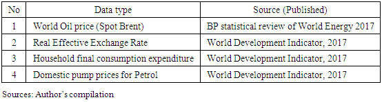
The data type in this study are secondary from 1993 to 2016. The details of the data types and sources in this study are presented in table 1 below.

Table 1. Data Type and Sources

3.1. Description of Data Set

The details of the data used in the study are presented below.

3.1.1. Domestic Pump Prices for Petrol

The study obtained data from the World Development Indicator 2017 of the World Bank. It has been assumed in the study that, lower world oil price would result into higher value of oil imported which eventually would result into lower domestic pump prices of oil during the period under consideration. Petrol has been used to represent domestic price because it used by rural (motorcycles) and urban households (motorcycles, commuter taxis and personal cars) in the daily transportation of persons hence having a big impact on the economy.

3.1.2. World Crude Oil Price

The study used spot price Brent as a proxy to world crude oil prices since is the most applicable to the study as it is widely used as a benchmark for crude oil pricing. According to EIA (2014), the most widely used benchmarks are associated with crude oil that has four common qualities: stable and ample production; a transparent, free-flowing market located in a geopolitically and financially stable region to encourage market interactions; adequate storage to encourage market development; and/or delivery points at locations suitable for trade with other market hubs, enabling arbitrage (profit opportunities) so that prices reflect global supply and demand. Further, it has been assumed in the study that lower world oil price would result into lower domestic pump prices. The data for Brent spot price was obtained from BP statistical review of World Energy 2017.

3.1.3. Real Effective Exchange Rate (REER)

The inclusion of real effective exchange rate (REER) in the model was vital since oil price on the world market is quoted in US dollars. Real effective exchange rate is the nominal effective exchange rate (a measure of the value of a currency against a weighted average of several foreign currencies) divided by a price deflator or index of costs.

In addition, any change in the exchange rate of the local currency against the USD affect the domestic price of oil and the real value of wealth and thus the demand for oil. Since Uganda is generally a net importer of crude oil and a price-taker, any changes in the exchange rate will influence demand for crude. An increase in REER implies that exports become more expensive and imports become cheaper and hence an increase indicates a loss in trade competitiveness. The quarterly data of Real Effective Exchange Rate (REER) Index (2010=100) were obtained from the World Development Indicator, 2017.

3.1.4. Household Final Consumption Expenditure

Household final consumption expenditure, Purchasing Power Parity (PPP) (constant 2011 international USD) is expected to increase national energy consumption through per capita consumption in key areas such as transportation. The data were obtained from the World Development Indicator 2017 of the World Bank.

3.2. Model Specification

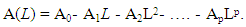
This study uses SVAR models to investigate the pass-through effect of world oil price shocks to domestic oil pump prices. The details are indicated below.

A VAR is an n-equation, n-variable model in which each variable is in turn explained by its own lagged values, plus (current) and past values of the remaining n-1 variables.

Following Raghavan (2015), the interactions between oil and macroeconomic variables can be described using an SVAR model

(1)

Where;

X_t is a (n x 1) vector of variables, X_t = (World oil price, Real effective exchange rate, Domestic pump prices for petrol, Household final consumption expenditure);

A_i is a (n x n) coefficient matrix for i = 0, 1, 2, p, which capture dynamic interactions between the variables in the model;

is (n x1) vector of serially uncorrelated structural shocks with properties, and

, where is a diagonal matrix containing the variances of the structural disturbances.

SVAR in (1) can be written as;

(2)

where A(L) is a matrix polynomial in lag operator L and

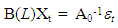
The reduced form VAR representation of (2) is;

(3)

where B(L) = A₀^-1 A(L) and,

The reduced form errors are related to the structural disturbances by;

(4)

Equation (4) can now be represented as;

(5)

The impulse response functions of the SVAR model can be derived from the Vector Moving Average (VMA) representation;

(6)

where

Since the structural shocks, are obtained by imposing appropriate restrictions based on economic theory and stylized facts on the contemporaneous matrix A₀ and on the lag matrixes B(L), the effects of these shocks on domestic variables can be captured more effectively through the impulse response function given in equation (6).

Following Odongo (2013) and Ito and Sato (2007), the analysis of the pass-through effect of oil price shocks to domestic pump prices for petrol can be presented as follows, basing on the relationship between reduced-form VAR residuals and the structural disturbances

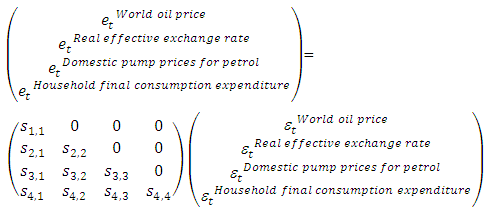(7)

The structural model is identified because the k(k −1)/2 restrictions are imposed on the matrix S as zero restrictions where k denotes the number of endogenous variables. The resulting lower-triangular matrix S implies that some structural shocks have no contemporaneous effect on some endogenous variables given the ordering of endogenous variables.

The arrangement/ordering of variables in the specification in equation (7) determines the structure of shocks. The first variable world oil price has an influential effect on all other variables below it, but it is not affected by any of these variables. The second variable real effective exchange rate gets an impact from the first variable. It doesn't have any impact on the first variable but it influences all other variables below it.

The third variable (domestic pump prices for petrol) is affected by both real effective exchange rate and world oil prices while it also affects the household final consumption expenditure.

The last variable, household final consumption expenditure receives impact from all the variables above it.

Using the structural VAR, the pass-through effect of oil price shocks to the domestic oil prices at horizontal lag was obtained by running Variance Decomposition and Accumulated Impulse Response with respect to an innovation of one standard deviation of shock.

3.2.1. Restrictions on Structural VAR Coefficients

Based on recursive approach, the decomposition of variance/covariance matrix of reduced form residuals was done on lower triangular matrix k(k-1)/2, where k is the number of variables. In a contemporaneous relationship of a four variables model as in this study, there are 6 restrictions {4(3)/2} required for identification of the effect of structural shocks on endogenous variables. Restrictions are imposed on this matrix to identify structural shocks in the case where shocks do not have any contemporaneous effect on endogenous variables (Siok & Zhanna, 2008).

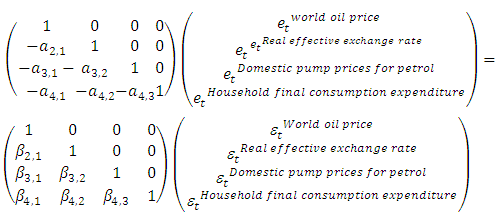(8)

As in Odongo (2013), restrictions on structural VAR coefficients were imposed on the structural error vector (ε_t) on the basis of economic theory. To obtain economically meaningful results from the VAR system, the price pass-through effect of world oil price shocks on domestic petrol/gasoline prices was estimated using specification that links reduced form random errors (et^{World oil prices}, et^{Real effective exchange rate}, et^{Domestic pump prices for petrol} and et^{Household final consumption expenditure}) with the structural errors (εt^{World oil prices}, εt^{Real effective exchange rate}, εt^{Domestic pump prices for petrol} and εt^{Household final consumption expenditure}).

Restrictions are imposed on the structural coefficients which guarantee that the outcome from the structural coefficients depicts the contemporaneous relationship between internal adjustments and unexpected exogenous shocks from world oil price. Restrictions on the structural coefficients indicated in this study are imposed on initial period only because all variables in this study are permitted to freely interact with each other in all periods following the one in which innovation took place.

Generally, this factorization explains the relationships between reduced shocks only in the first period, while later every shock can be affected by any other shock. This means that coefficients presented in the matrix (8) are all equal to zero.

As in Kumah and Matovu (2005), coefficients -a_2,1; -a_3,1; -a_3,2; -a_4,1; -a_4,2 and -a_4,3 on the left side of matrix (8) show the workings of internal adjustment (automatic stabilizer) due to external shocks, while the diagonal coefficients on the right hand side of matrix (8) capture the workings of external shocks due to structural innovation represented by shocks from world oil price real effective exchange rate domestic pump prices for petrol and household final consumption expenditure

It assumes, from the point of view of automatic stabilizers, a time lag between world oil price innovations and changes in real effective exchange rate (REER), domestic pump prices and household final consumption expenditure. The matrix in equation (8) therefore shows the contemporaneous relationship between internal adjustments and unexpected exogenous shocks from world oil price. It is further noted that variance decomposition analysis and accumulated impulse response functions were all estimated as per the above restrictions.

The benefit of using structural VAR specification in this study is that it solves the endogeneity problem that can occur under a single equation approach. Secondly, this technique applies restrictions on the structural coefficients that identify structural shocks from the VAR system (Odongo, 2013).

3.3. Data Estimation Techniques

This section describes the general technique used in the study.

3.3.1. The General Approach

E-views software was used to estimate the time series data. The data for analysis was considered from 1993 to 2016. The choice of the sample period was based on data availability of selected series in the required frequency. The annual data was converted to quarterly data using E-veiws (using quadratic-match average method). According to E-views (2017a), frequency conversion from low to high and from high to low is a powerful task that is performed with its software perfectly. The study carried out a number of analysis which includes; Stationary test using Philips Perron (PP) and Kwiatkowski, Phillips, Schmidt and Shin (KPSS) test, Co-integration test using Johansen Co-integration test method, Variance decomposition of SVAR, accumulated impulse responses of SVAR, Autoregressive Conditional Heteroskedasticity(ARCH) Test and Regression Specification Error Test (RESET). The optimum lag has been determined by comparing every lag to the criteria used (Schwarz Information Criterion) and choosing the minimum values from the information criteria.

3.3.2. Stationary Test

The stationarity test in this study used regressions of time series data analyzed against a constant. These regressions were expressed as follows;

(9)

(10)

The stationarity of residuals (ε_t) were tested.

The series were examined for stationarity using Philips Perron (PP) test and Kwiatkowski, Phillips, Schmidt and Shin (KPSS) test using a lag selected by Schwarz Information Criterion (SIC). The first step in determining stationarity involved graphing the data to observe its behaviour. The next step involved conducting a unit root test. The null hypothesis of PP is that the series has a unit root (non-stationary) and rejecting the null hypothesis of the PP unit root test implies the series is stationary. The null hypothesis of the KPSS test is that the series stationary and rejecting the null hypothesis of the KPSS stationarity test implies the series is non- stationary. KPSS test for stationary around a deterministic trend (that is, trend-stationary).

3.3.3. Cointegration Test

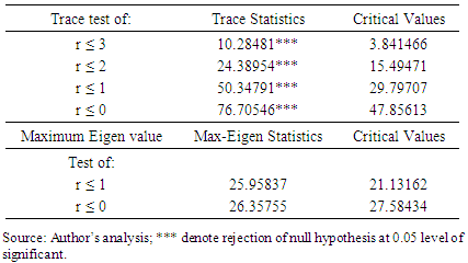
The necessary criteria for stationarity among non-stationary variables is called cointegration. Testing for cointegration is necessary step to check if one is modelling empirically meaningful relationships. For this study, Johnsen test procedure was adopted to test for cointegrating relationship within endogenous variables based on Maximum Likelihood (LM) test and unrestricted Vector Auto Regression (VAR) test. Cointegration rank r (number of cointegrating vectors) was tested using trace statistics and Maximum Eigen Statistics (MES).

3.3.4. Variance Decomposition

Knowledge of forecast errors is useful in determining the relationship between variables. Variance decomposition separates the variation in an endogenous variable into the component shocks to the VAR. Hence, the variance decomposition provides information about the relative importance of each random innovation in affecting the variables in the VAR (E-views, 2017b). As in Odongo (2013), variance decomposition in a structural VAR indicates the amount of information each variable contributes to other variables in an autoregressive manner and further determines the amount of forecast error variance that can be explained by exogenous shocks. These were estimated from SVAR models in this study. The results of the variance decomposition were interpreted once generated.

3.3.5. Accumulated Impulse Response Function

As in Odongo and Muwanga (2014), the accumulated impulse responses of endogenous variables captured dynamic responses of endogenous variables due to one standard deviation in structural innovation. Restrictions imposed on the structural coefficients which allowed for a transformation process that uncovers shocks from the VAR system. These were estimated from SVAR models in this study.

4. Presentation and Discussion of the Results

The results of this study are obtained from the estimates of variance decomposition and accumulated impulse response functions of endogenous variables. Details of the results are presented below.

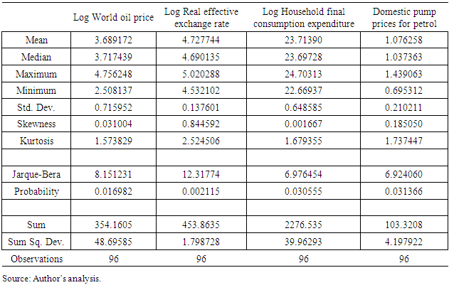
4.1. Descriptive Statistics

The analysis on descriptive statistics has been carried out in this study to find the relationship between the variables in the model specified. The details of which are indicated in table 2 below. The summary statistics in table 2 below indicate that normality test has been rejected in all the 4 variables at 5 percent level of significance. The non-normality could have been caused by excess kurtosis. The study proceeds with stationarity test on the variables using unit root test.

Table 2. Descriptive Statistics

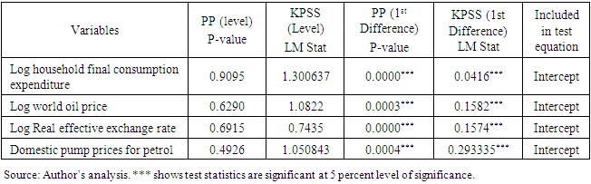
4.2. Test for Stationarity

The stationarity test has been carried out using Philips Perron (PP) and Kwiatkowski, Phillips, Schmidt and Shin (KPSS) test. The summary of the stationarity test is presented in table 3.

The results in table 3 show that using PP and KPSS tests, all other variables are non-stationary at levels at 5 percent level of significance. In their first difference, all the variables are stationary at 5 percent level of significance. The study proceeds to test for cointegration among the variables under study. The stationary variables are shown in the figure 5 below.

Table 3. Stationary Test for Variables under Study

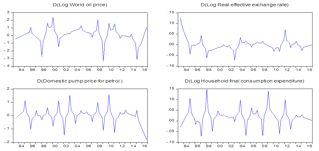Figure 5. Variables in their stationary form

4.3. Test for Cointegration

Cointegration test has been carried out in this study to determine if there exists any long-run relationship within variables in the model specified. The results for the Johansen cointegration test carried out in the study are presented in table 4 below.

Table 4. Cointegration Test Results

The results from Unrestricted Trace Statistics (UTS) in this table indicate four cointegrating vectors at 0.05 percent level of significance; while the results from Maximum Eigen Statistics (MES) in the same table also indicate no co-integrating vectors at 0.05 percent level of significance Thus; there exists a long run relationship within variables in the model specified. Even though there were cointegrating relationships within endogenous variables in the model, structural VAR model was selected for the study because it best explains feedback effect among a set of variables (Odongo and Muwanga, 2014).

4.4. Diagnostic Test

Following the cointegration test carried out in this study, the study proceeds to carry out Autoregressive Conditional Heteroskedasticity (ARCH) test to determine whether there exists serial correlation in the variables specified in the study and finally, the study carried out Regression Specification Error Test (RESET) to determine whether there exists misspecification error among the variables specified in the study. Details of the diagnostic test carried out in this study are indicated below.

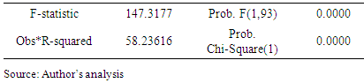
4.4.1. Autoregressive Conditional Heteroskedasticity (ARCH) Test

The ARCH test uses autocorrelations and partial autocorrelations of the squared residuals to determine whether there exists any serial correlation in the residual of the variables in the model specified. Details of the results from the ARCH test carried out in this study are presented in table 5.

Table 5. Heteroskedasticity Test: ARCH

A small p-value (typically ≤ 0.05) indicates strong evidence against the null hypothesis, meaning rejecting the null hypothesis. Under the null hypothesis of no ARCH up to order 1 in the residuals, the probability of rejecting Ho is 0.00. At 1 percent level of significance, this study, therefore, reject the null hypothesis of no ARCH in the variables in this study.

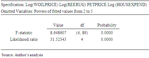
4.4.2. Regression Specification Error Test (RESET) for Misspecification

Regression Specification Error Test (RESET) has been carried out in this study to test for specification error in the variables specified in the study. Details of the results from the RESET test in this study are indicated in table 6 below.

Table 6. Ramsey RESET Test

The RESET F-statistic has a p-value of 0.00 percent and Likelihood ratio has a p-value of 0.00 percent, indicating that the null hypothesis has been rejected at 1 percent level of significant. A small p-value (typically ≤ 0.05) indicates strong evidence against the null hypothesis, meaning rejecting the null hypothesis.

Following the RESET, the study proceeds to estimate the AR characteristic polynomial to check on the stability of the SVAR.

4.4.3. AR Characteristic Polynomial

As seen in figure 6, all the roots lie in the unit circle, hence the SVAR model is stable. The study proceeds to estimate variance decomposition and accumulated impulse responses in the next sections.

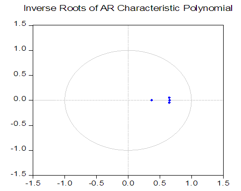Figure 6. AR Characteristic Polynomial

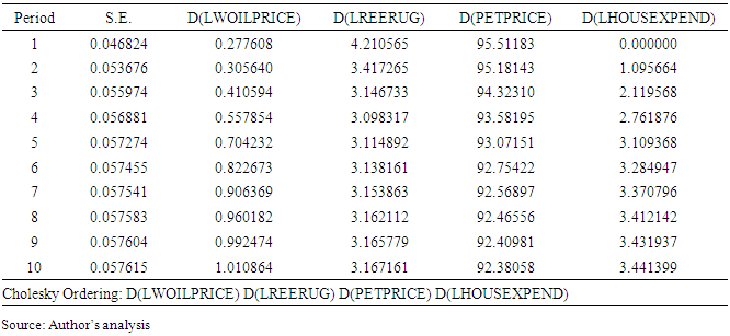
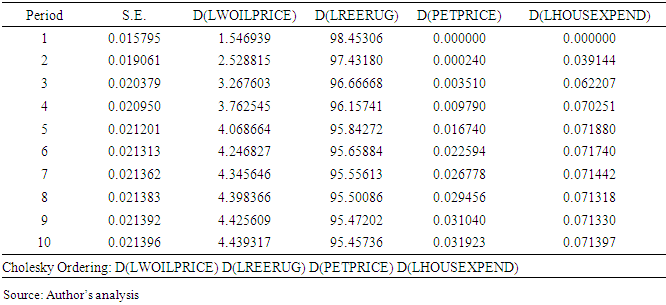
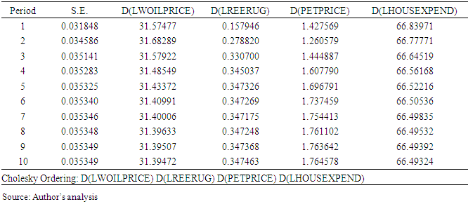
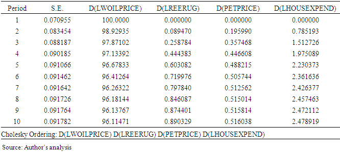
4.5. Variance Decomposition

Variance decomposition analysis has been carried out for domestic petrol pump prices to estimate the relative importance of each endogenous variable. The result is shown in table 7 below.

Table 7. Variance Decomposition of domestic petrol/ gasoline prices

As per the results in table 7 below, 92.4 percent of total variation in domestic petrol prices are explained by itself over the whole sample period, 3.4 percent of total variation in domestic petrol prices are explained by shocks from household final consumption expenditure, 3.2 percent of total variation in domestic petrol prices are explained by shocks from real effective exchange rate while 1 percent of the total variations in domestic petrol prices are explained by world oil price. However, household final expenditure is seen to affect domestic pump price for petrol more compared to other variables under study.

Following the results above, there is an insignificant pass-through effect of world oil price shocks to domestic oil prices in the period under review since quite a huge percentage of total variations in the domestic petrol prices are explained by itself while only 1 percent is explained by shocks from world oil prices.

There is also a likelihood for total variation in the real effective exchange rate in the period under study to affect the performance of domestic pump price for petrol, such that a positive variation in real effective exchange rate increases the import of oil products thereby making domestic pump prices of petrol to fall.

A negative variation in real effective exchange rate decreases the import of oil products thereby making domestic pump prices of petrol to rise. The variance decomposition of the real effective exchange rate (REER) with respect to other endogenous variables has been estimated in line with the above arguments and the results are presented in table 8.

Table 8 below shows that that quite a huge percentage (95.5 percent) of total variations in REER in Uganda are explained by itself over the whole sample period, while only 4.4 percent of the total variations in REER are explained by shocks from world oil price, 0.07 percent from household final consumption expenditure and finally 0.03 percent from domestic petrol prices. However, world oil price is seen to affect REER more compared to other variables under study.

Table 8. Variance Decomposition of Real Effective Exchange Rate (REER)

There is also a possibility for total variation in household final consumption expenditure to affect the performance of domestic pump price for petrol, such that a positive variation in household final consumption expenditure increases domestic demand for petrol thereby increasing the domestic pump prices of petrol. The variance decomposition of household final consumption expenditure has been estimated in line with the arguments and presented in table 9. The results in table 9 shows that quite a big percentage of 66.5 percent of total variations in household final consumption expenditure in Uganda are explained by itself over the whole sample period, while 31.4 percent of the total variations in household final consumption expenditure are explained by shocks from world oil price, 1.8 percent from domestic petrol prices and finally 0.35 percent from real effective exchange rate. However, the world oil price is seen to affect household final consumption expenditure more compared to other variables under the study.

Table 9. Variance Decomposition of Household Final Consumption Expenditure

Finally, there is also a possibility for total variation in world oil price to affect the performance of domestic pump price for petrol, such that a positive variation in world oil prices increases the domestic pump prices of petrol. The variance decomposition of world oil price has been estimated in line with the above arguments and presented in table 10 above. The results in table 10 above shows that quite a huge percentage of 96.1 percent of total variations in world oil price are explained by itself over the whole sample period, while 3.9 percent of the total variations in world oil prices are explained by shocks from other endogenous variables under study.

Table 10. Variance Decomposition of World Oil Prices

Following the estimated results in table 7, 8, 9 and 10, it can be concluded that the performance in domestic pump price for petrol in the period under study has not been determined by world oil price and neither by real effective exchange rate and household final consumption expenditure, rather by other factors operating within the economy. Such factors may be domestic taxes, collusion in pricing by petroleum importers since the market is dominated by a few big importers/retailer. Further, household final expenditure and REER is seen to affect variations in domestic pump price for petrol more compared to other variables under study.

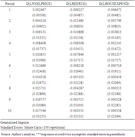
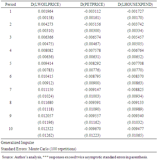
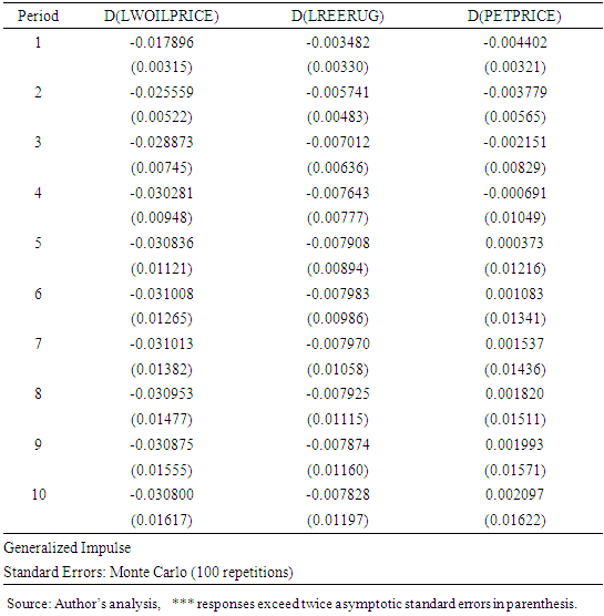
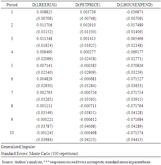
4.6. Estimates of Accumulative Impulse Responses

Table 11, 12, 13 and 14 below presents the results from the estimates of the accumulative impulse response function of domestic prices (petrol/gasoline), real effective exchange rate (REER), household final consumption expenditure and world oil price due to shocks from other endogenous variables. The responses are from contemporaneous shocks and on-word through the whole sample period. The magnitudes of the shocks are in the first row while their standard errors are in parenthesis in the second row.

As shown in table 11 below, the estimated responses of world oil price shocks, real effective exchange rate (REER) and household final expenditure do not exceed the two standard error criteria of significance in the whole period. The estimated responses of the accumulative impulse response of domestic pump prices for petrol in this table 11, therefore, indicate that there is an insignificant pass-through effect of world oil price shocks to domestic pump prices for gasoline/petrol.

Table 11. Accumulative Impulse Response of Domestic Petrol/gasoline Prices

There is also a likelihood for total variation in the real effective exchange rate in the period under study to affect the performance of domestic pump price for petrol/gasoline, such that a positive variation in real effective exchange rate increases the import of oil products thereby making domestic pump prices of petrol to fall. The accumulative impulse response of real effective exchange rate with respect to shocks from other endogenous variables has been estimated in line with the above arguments and the results are presented in table 12.

As in table 12 below, there exist insignificant responses from real REER due to shocks from other endogenous variables throughout the whole sample period. The estimated responses of world oil price shocks, domestic petrol prices and household final consumption expenditure do not exceed the two standard error criteria of significance in the whole period.

Table 12. Accumulative Impulse Response of Real Effective Exchange Rate (REER)

Table 13. Accumulative Impulse Response of Household Final Consumption Expenditure

There is also a possibility for total variation in household final consumption expenditure to affect the performance of domestic pump price for petrol, such that a positive variation in household final consumption expenditure increases domestic demand for petrol thereby increasing the domestic pump prices of petrol. The accumulated impulse response of has been estimated in line with the above arguments and presented in table 13 above.

As shown in table 13 above, the estimated responses of world oil price shocks, real effective exchange rate (REER) and domestic prices for petrol do not exceed the two standard error criteria of significance in the whole period.

The result presented in table 13, therefore, show that there exist insignificant responses from household final consumption expenditure due to shocks from other endogenous variables throughout the whole sample period.

Table 14. Accumulative Impulse Response of World Oil Price

Finally, there is also a possibility for total variation in world oil price to affect the performance of domestic pump price for petrol, such that a positive variation in world oil prices increases the domestic pump prices of petrol. The accumulated impulse response function of the world oil price has been estimated in line with the above arguments and presented in table 14 above.

As shown in table 14 above, there exist insignificant responses from world oil prices due to shocks from other endogenous variables throughout the whole sample period. The estimated responses of the real effective exchange rate, domestic petrol prices and household final consumption expenditure do not exceed the two standard error criteria of significance in the whole period.

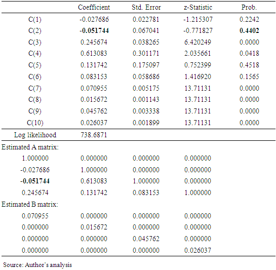
4.7. Estimates of the Structural VAR Coefficients of Matrices A and B

The structural VAR estimates for matrices A and B is shown in table 15 and it summarizes the SVAR results for this study. Matrix A shows internal adjustments due to external shocks from world oil prices represented by matrix B and this is further indicated by equation 8.

Table 15. Estimates of the Structural VAR Coefficients of Matrices A and B

As shown in table 15, the effect of world oil price on real effective exchange rate (C1) and domestic pump prices for petrol (C2) are negative and insignificant. Furthermore, the effect of real effective exchange rate on household final consumption expenditure (C5) is positive but insignificant. Finally, the effect of domestic pump prices for petrol on household final consumption expenditure (C6) is also positive but insignificant.

Thus the results from the Structural VAR coefficient in this study therefore indicate insignificant pass through effect of world oil price shocks to domestic pump prices. This result is in line with our earlier findings from Variance Decomposition analysis and Accumulative Impulse responses. This study can categorically confirm that there is insignificant pass through effect of world oil price shocks to domestic pump prices in the period under the review.

5. Conclusions

The study investigates the pass-through effect of world oil price shocks to the domestic pump prices for petrol in the period between 1993 and 2016 using the SVAR model. The results from the estimates of variance decomposition, accumulated impulse responses and the SVAR coefficients in this study are consistent with each other. The above results indicate an insignificant pass-through effect of world oil price shocks to domestic pump price for petrol in the period under study.

The results, therefore, show that performance in the domestic pump price for petrol/gasoline in the period under study has never been determined by world oil price, neither has it been determined by real effective exchange rate nor household final consumption expenditure but rather been determined by other operating factors in the economy. Such factors may include nature of domestic taxes and collusion in pricing by petroleum importers since the market is dominated by a few big importers/retailer.

6. Policy Implications

The economy should be structured in such a way that changes in world oil price can easily be transmitted in to the domestic pump prices.