1. Introduction

Many African countries are endowed with abundant natural resources. However, these countries, especially in Sub Sahara Africa, are faced with abject poverty and lack of sufficient skilled labor (human capital), food and financial crises, political tensions and debt burden which lead to debt overhang. Debt overhang inhibits investment and growth as the government’s debt burden imposes an implicit tax on the private sector [1].

Despite all the factors that hampered development for many years, starting from the mid 1990s, many economies of Sub-Saharan Africa have achieved promising growth that was robust from 2005 upwards [2]. The main reasons for growth in most African countries, include primary production and foreign trade, especially export trade [3].

South Africa, as a developing country needs to have a well functioning external sector that can enable her to have competitive export and favorable investment climate to attract more foreign capital and technology.

2. Literature Review

2.1. Theoretical Analysis

The relationship between trade and economic growth has drawn attention to many academics and practitioners in both developing and developing countries. For academics, the main curiosity has been on the causality phenomenon, whether trade drives economic growth or it is economic growth which leads to trade or the two reinforce each other. So a number of scholars have attempted to investigate the nexus between trade and growth, and their related themes such as trade openness and economic growth, while others have researched on the role of the components of trade (export and import) on economic growth [4].

Exports and imports of goods and services play a vital role in economic development as exports require companies to be innovative enough to maintain market share. Consequently, exports lead to increased sales and therefore more profit to the exporting companies resulting from an increased market share [5]. Export Led Growth (ELG) leads to efficient allocation of resources, hence playing a significant role in a country’s economic development [6].

According to neoclassical economists, there is strong association between trade expansion and economic growth. Export growth accelerates economic growth through economies of scale; stimulating supply and demand in the economy [7]. In theory, export growth promotes economic growth, which leads to skill formation and technological progress. Exports provide a good way of entering international markets and expanding the manufacturing sector. It is an efficient means of introducing new technologies both to the exporting firms in particular and to the rest of the economy, and providing a mechanism for learning and technological advancement [8]. South Korea, China, India and Honduras serve the best example in delineating export-led growth [9-12].

However, in some cases, exports may not lead to the desired outcomes. Existence of unforeseen competition, political instability of the trading partners leading to wars and civil unrest, unpopularity of the products or bilateral trade relations may hamper exports. On the other hand, imports lead to exit of local currency, aggravating a country’s Balance of Payment deficit hence affecting economic growth. But, in other cases, import can lead to economic growth, especially for the case of import of machinery and electronic equipment. Therefore, there has been a persistent debate among academic and researchers as to whether it is export or import that promotes a country’s economic growth [5].

2.2. Empirical Literature Review

The Export-led growth hypothesis (ELGH) is based on the idea that exports drive economic growth [13]. From the methodological approach, empirical literature on export, import and economic growth nexus can be categorized into two broad groups.

The first category uses cross-sectional approach to test the economic theory about export and economic growth nexus by using rank correlation approach, ordinary least squares (OLS) method, 2 stage least squares (2SLS) and random effect estimation method [14]. The results from such studies conducted in different countries have shown a positive relationship between exports and economic growth [15-19]. In 1985 David Jaffe conducted a panel study to investigate export dependency and economic growth for both developed and developing countries. In his study he came up with two major findings; first, export dependence has a significant positive effect on economic growth. Secondly, the positive relationship between export dependence and economic growth is reduced, and even reversed, when a set of structural conditions formulated in export reliance and “vulnerability” theses is specified empirically [20]. Therefore, the study suggests a more careful specification of the theoretical relationships associated with export dependence/world-economy theory. In a bid to find out how the product and the destination structures of exports shape the growth dynamics for European countries, Ribeiro et al, studied 26 European union member countries and found that growth is fostered through export specialization in high-value added products such as manufacturing and high technology, and by export diversification across partners [21]. Also, Saglam and Egeli used dynamic panel data analysis to compare domestic demand and export-led growth strategies for sixteen European transition economies from 1990 – 2015 [22]. Their study revealed a bilateral relationship between export and growth.

The second category of researchers has used the time series approach. Earlier studies of this approach were mainly based on Granger’s (1969) and Sims (1972) causality methods. There is a myriad of time series literature on export, import and economic growth [23-26]. Since these studies did not take into account the cointegration properties in their estimation, they have not been able to support the export-led growth (ELG) hypothesis. One of the recent studies was an investigation on the validity of the ELG hypothesis for Malaysia by using the vector error correction model (VECM) approach for time series from 991:Q1 to 2012:Q4. The study finding was that the ELG hypothesis applies to Malaysia in the long run [27]. Moreover, Ali and Li conducted a comparative study on the ELG hypothesis for China and Pakistan using the autoregressive distributed lags (ARDL) and Granger causality approach. Their study found that there is supporting evidence for the ELG hypothesis for the two countries [28].

2.3. Empirical research on ELG in Africa

A number of studies have shown that exports have positive impact on the economies of developing countries, including Africa. The studies differ in their coverage and methodologies spanning from panel, time series and qualitative approaches. In a study covering twenty eight African countries, Fosu (1990) used pooled regression method and found that there is positive relationship between exports and economic growth. In 1991 a couple of researchers conducted a study on export instability and economic growth for a panel of 34 Sub-Sahara African countries for the period 1960-1986. By using the neoclassical growth equation, after allowing for effects of other variables on economic growth, he found that export instability has a negative and significant effect on economic growth rate in Sub-Saharan African countries [30]. In 2011, another group of researchers used the Generalized Method of Moments (GMM) estimation to investigate the relationship between real per capita income and agricultural/manufactured exports in 35 countries in Sub-Sahara Africa. The results showed a positive impact of agricultural exports on per capita income of the countries under their study [31]. Using a combination of approaches, in 2014 an empirical study on the ELG hypothesis covering 30 African countries for the period between 1990 and 2005 was conducted [32]. The panel data approaches included pooled OLS, fixed effects model (FE), random effects model (RE), Two-Stage Least Squares (2SLS); and found a positive relationship between exports and economic growth in the countries under study [32]. Likewise, [33] used a new generation panel data approach to analyze the ELG for the selected countries in Sub Sahara Africa, and found positive results supporting the ELG hypothesis for Sub Sahara African Countries.

In a time series study that involved regression of GDP growth against the growth rates of capital, labor, fuel exports, non-fuel primary products, consumption and government consumption it was concluded that low income countries of Africa can use non-fuel primary products as the major engine of economic growth [34]. In developing the idea of Ukpolo [34], Abogan [35] investigated the role of non-oil export and economic growth in Nigeria. They utilized time series data covering the period between 1980 and 2010 and found that there was moderate impact of non-oil export on the economic growth of Nigeria [35]. Also, a study on the role of exports in economic growth in Namibia, using time series data ranging between 1968 and 1992 found evidence of causal relationship between export and economic growth, although there was no discernible sign of accelerated economic growth because of export. Most importantly, it was found out that domestic export supply factors are more important to growth than external demand factors [36].

For the case of South Africa, a time series study covering the period between 1964 and 1993 using cointegration and Granger Causality procedures, showed that exports does not Granger cause economic growth [37]. However, another study showed that there was Granger causality running from export to economic growth [38]. A more recent work on the causal relationship between export, import and economic growth was conducted by Moroke and Manoto [39]. These researchers used time series data ranging between 1998 and 2013 and found that there was a significant Granger causality running from exports and imports to GDP and from imports to exports [39].

The earlier researchers in South Africa have covered short periods, for example, between 1964 and 1993 [34] and the the other study covered the period between 1998 – 2013 [39]. They specifically examined the effects of exports to GDP in South Africa in the period in question and found contradicting results. While [34] found that exports do not Granger cause economic growth, [39] found that there is Granger causality running from exports to economic growth. Therefore, in our study we would like to cover a bigger sample, to include all time series data that is available for the period between 1961 and the most recent annual period, that is 2017, so that we can more clearly see the impact of export in economic growth in South Africa.

Moreover, although [39] have indicated the direction of causality between exports and imports, they have not shown to what extent each variable impacts on economic growth. In that regard, through variance decomposition, we shall attempt to show the extent of influence of each of these variables to economic growth of South Africa.

3. Motivation

The role of export in economic growth cannot be overemphasized. However, developing countries, especially in Sub-Sahara Africa are still lagging behind in reaping the benefits accrued from export trade. Therefore, it is important to study this area and make good analysis so as to inform decision makers who shall formulate sound policies regarding exports and international trade in general. In this paper we shall investigate the ELG approach with an inclination to South Africa, covering the period 1961-2017. Choice of this country is based on the fact that South Africa ranks at the top in terms of export performance in Africa. In 2017, for instance, South Africa’s exports were valued at US$88.3 billion, making about 21 per cent of total exports from the continent as a whole. Therefore, we expect to have better access to information and obtain the required amount of data in order to make meaningful analysis and arrive at better conclusions.

4. Methodology

4.1. Data

In this study we used secondary macroeconomic data based on availability, starting from the earliest to the latest that we could obtain. Therefore, annual time series data was taken covering the period 1961 - 2017, with a total of 57 observations for each variable. All the variables (exports, imports and GDP) were obtained from the World Bank’s World Development Indicators’ database (WDI). The variables were in percentages.

4.2. Estimation Techniques

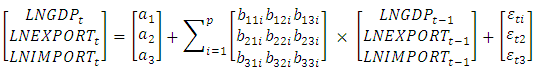
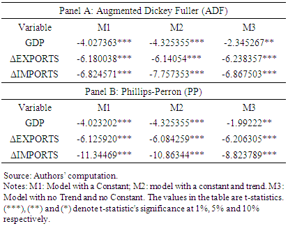
Our empirical investigation involved three steps. The first step was to examine the Stationarity of the variables through unit root tests. We conducted the Augmented Dickey Fuller test (ADF, 1979) and the Philips-Perron (1988) unit root tests.

The second step involved checking the presence of long-run relationships between the variables. The ARDL bounds testing approach [40] was employed to serve this purpose.

In the third step we investigated the causal relationships among the variables using the Toda-yamamoto [41] approach. This approach is especially useful in a situation where the variables are I (0) and I (1). If variables are not integrated of the same order (as seen in our case) the wald test statistic (the conventional approach) would not follow its usual asymptotic chi-square distribution under the null. In that similar case, where we have our variables of I (0) and I (1), testing for Granger non-causality from the conventional Vector error correction method would not be proper.

The ARDL approach, adopted in our second step, has become the most popular approach amongst the 21st generation researchers in economics and econometrics and related studies that involve analysis of time series data. This is because; the ARDL approach has some added advantages when compared with other approaches. ARDL approach helps to do away with the problem of endogeneity, especially in macroeconomic time series, it can be applied to test long run relationships regardless the order of integration of the time series, that is, I(0) I(1)), but not I(2) of course [42].

The ARDL bounds testing approach to cointegration (Pesaran, et al, 2001) was based on the following equations:

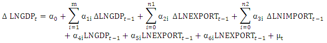(1)

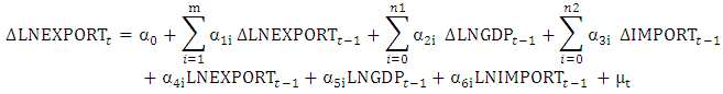(2)

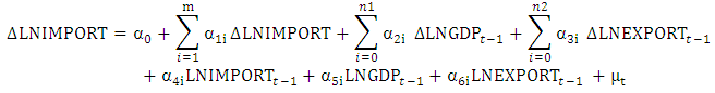(3)

Where: LNGDP = log of GDP; LNEXPORT=log of Export; LNIMPORT = log of imports; The m represents the optimal lag of the dependent variable and n1 and n2 represent the optimal lag orders of the regressors; Δ is the first difference operator and μ = the uncorrelated white noise error term.

The next step was to perform an F-test of the hypothesis, H₀: ⍺₃=⍺₄=0; or δ₃=⍺₄=0 against the alternative that H₀ is not true. So we had to check for the absence of long-run equilibrium relationship between the variables. A rejection of the null means that we have a long run relationship, while failure to reject the null hypothesis implies that there is no long run relationship between the variables in question.

Pesaran et al (2001) provides bounds on the critical values for the asymptotic distribution of the F-statistic with respect to the lower and upper bounds on the critical values. In each case, the lower bound is based on the assumption that all of the variables are I (0) and the upper bound is based on the assumption that all of the variables are I (1). If the computed F-statistic falls below the lower bound we would conclude that the variables are I (0), meaning that there is no cointegration; but if the F-statistic exceeds the upper bound, we conclude that there is cointegration. In case the F-statistic falls between the bounds, the test is inconclusive (Pesaran, et al, 2001). In eviews-10 the ARDL model is embedded in the system, so this task can be performed straight away by choosing the ARDL option in the estimate equation and then, after generating the output, the F-statistic as well as its critical bounds are obtained by looking at the long run form bounds testing results.

Furthermore, the ARDL bounds testing procedure is sensitive to the selection of the lag structure (m, n). In this study, maximum lag length on each variable was set to five and the optimal lag structure was selected using the Akaike Information Criterio (AIC). The results of lag selection procedure are reported in table 3.

The model was also subjected to all the diagnostic tests for serial correlation, heteroscedasticity and normality as well as stability tests.

4.3. Causality Test

Conventionally the Wald test would be used to test linear restrictions on the parameters of a VAR model. However, in a case where the variables are I (0) and I (1), the Wald test statistic would not follow its usual asymptotic chi-square distribution under the null. In that similar case, where we have our variables of I (0) and I (1), testing for Granger non-causality from the conventional Vector error correction method would not be proper. Instead, we adopted the Toda and Yamamoto’s (1995) approach of testing for Granger non-causality using standard vector auto regression (VAR). We first selected the optimal lag order for the endogenous variables and declared the extra lag of each variable to be an exogenous variable, and estimated an unrestricted VAR. Then we performed residual diagnostic tests to see if our results suffered from serial correlation and finally tested for stability of our system by looking at the modulus of the unit root as well as its resulting inverse root characteristic polynomial.

In testing for Granger causality we estimated a VAR model of the form:

Then test H₀:b₁ = b₂ = b₃= 0, against H_A: H₀ is not true, implying that X does not granger cause Y.

5. Empirical Analysis

5.1. Descriptive Statistics

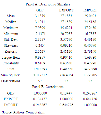
The summary in table 1 provides descriptive statistics and correlation of the variables. It shows that the series have 57 observations for each. By looking at the standard deviations it shows that IMPORT has the highest value (4.4915) and hence, highest variability of all variables, GDP (2.3557) and EXPORTS (3.5767). Also, IMPORT has the largest Kurtosis (2.7919) of all our variables.

Table 1. Summary Statistics

In addition, the table’s panel of correlation matrix indicates a positive relationship between GDP and EXPORT. A positive correlation between export and GDP can be in line with the Export-Led growth hypothesis, growth-led growth hypothesis or a two-way causality between export and GDP. However, at this stage we can not ascertain any causation since “correlation does not imply causation” [43, 44].

More so, the descriptive statistics output shows that the p-value of the Jarque-Bera tests for both series are statistically insignificant (> 5%), that is, all the values were sampled from a population that follows a Gausian distribution.

Generally, the descriptive output provides a quick picture of the data. This gives some important insight for one to carry out a more careful statistical analysis.

Results from the Augmented Dickey Fuller (ADF) tests show that our series are integrated of order zero and order one, I(0) and I(1). Neither of them was integrated of order two, I (2).

Also, Phillips-Perron (PP) unit root test results show that the variables are integrated of order zero and one, I (0) and I (1). Table 2 presents a summary for the unit root tests.

In order for standard cointegration testing (such as Engle and Granger, or Johansen) to make sense, it must be ensured that the series in question are integrated of the same order. However, in this particular case, it is not so. Our series are integrated of different orders, namely, I (0) and I (1), but, in any case, they are not I (2). So in such a scenario the ARDL/Bounds Testing approach is appropriate (Pessaran, et al, 2001).

Table 2. Unit root test results

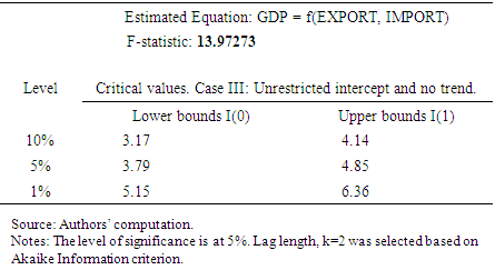
5.2. Results from the ARDL Long Run form and Bounds Testing

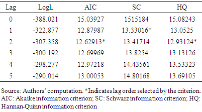
ARDL models can be estimated using either the standard least squares techniques or the built-in object equation in e-views. In this study, we used both, the Eviews 10 built-in equation object specialized for ARDL model estimation as well as the standard OLS method. The aim for this combination of methods was to validate findings from either of them, so as to ascertain our bounds testing results.

However, the results reported in this paper are based on the OLS estimations. But before that we ran an unrestricted VAR model in order to obtain the optimal number of lags to be used (table 3).

Table 3. Optimal Lag Selection

We initially set in the standard VAR with 5 lags for each endogenous variable; eventually the system picked lag 1 as the optimal lag based on Akaike Information Criterion (AIC). The ARDL bounds testing results are reported in table 4.

Table 4. Summary results of the ARDL bounds testing for cointegration

From the ARDL bounds testing results, the F-statistic, when GDP was the dependent variable, was 13.97273. This exceeds the critical values of the upper bounds (Pessaran, et al, 2001) at 10%, 5% and even 1% levels in the pesaran’s table (Case III: unrestricted intercept and no trend, Pessaran, et al, 2001, pp.300). Therefore, we have a compelling reason to conclude that when GDP is the dependent variable there is cointegration among the variables (exports, imports and GDP).

Also, the results show that, at 5%, all diagnostic tests are not violated by our models, that is, there is no serial correlation, no heteroscedasticity and the Jarquebera test shows that there is normal distribution. Moreover, both CUSUM and CUSUM of Squares tests show that the system is stable at 5 percent.

5.3. Causality Test Results

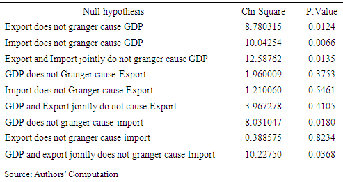
As it was pointed out in the methodology section, we have decided to adopt the Toda and Yamamoto’s (1995) approach of testing for Granger non-causality.

We maintained the same optimal lag order for the endogenous variables (table 3) and declared the 3^rd lag of each variable to be an exogenous variable, and estimated an unrestricted VAR.

The residual diagnostic tests showed that the resulting VAR did not suffer from serial correlation. Also, the inverse roots of Auto Regressive (AR) characteristic polynomial confirmed that our VAR system was stable (figure 1). The causality results are reported in table 5.

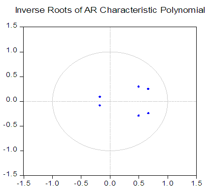Figure 1. Inverse roots of AR polinomial

Table 5. Granger Non-causality

From table 5, of the results), the null of no causality from export to GDP cannot be rejected. By the same token, causality from import to GDP cannot be rejected, implying that there is causality from export and import to GDP in Granger’s sense. Also, it shows that both export and import jointly causes GDP in granger’s sense. The table also shows that GDP causes import and that GDP and export jointly causes import.

However, the results of Granger causality tests are not exhaustive since they do not show the degree and magnitude of causality among the variables (Wolde-Rufael, 2009). Apparently, variance decomposition had to be used so as to explain the phenomenon in a better way.

Through variance decomposition analysis (presented in table 6), it shows that about 80% of the variations in economic growth are explained by shocks to economic growth in the short run, while in the long-run about 66%, 9% and 24% of the variations are explained by economic growth, exports and imports, respectively.

Table 6. Variance Decomposition of the variables

More so, the impact of exports to GDP is relatively smaller than the impact of imports. Also, the variation in exports in the short-run is explained by shocks to exports (about 96%), while in the long-run the variations are explained by exports (78%) as well as economic growth (18%) and imports (3%).

Finally, about 54% of the variations in imports in the short-run are explained by imports, while about 38% and 11% of the variations are caused by GDP and exports respectively. In the long-run, the variations in imports are caused by economic growth (48%) as well as imports (26%) and exports (about 24%).

6. Conclusions and Policy Implications

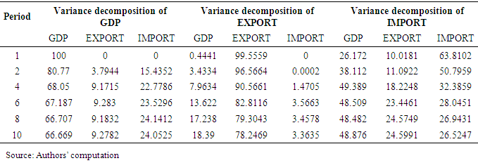
In this paper we conducted the empirical analysis of the export growth analysis for South Africa using the ARDL bounds testing approach adopted from Pessaran et al (2001). Furthermore, we carried out the Granger-non-causality analysis as per Toda and Yamamoto’s approach (1995). In all cases, optimal lag selection was based on Akaike Information Criteria.

It was found that export Granger causes GDP and the vice versa was not true. These results are similar to a study conducted by other scholars as well about the ELG hypothesis in South Africa (Rangasamy, 1985; Ziramba, 2011). Also, there was bidirectional causality between imports and economic growth in Granger’s sense, although our main attention was to examine the ELG hypothesis only. Furthermore, the results show bidirectional causality between imports and GDP in granger’s sense.

Having established the long-run relationship as well as the direction of causality between export and GDP in South Africa, one of the policy implications is that the ELG hypothesis applies in the country. Therefore the country should continue to promote export trade since it will bring the desired economic growth as well as labor creation and capital formation.

However, when comparing the degree of influence between exports and imports to GDP, through variance decomposition it shows that imports have a relatively bigger influence than exports to South Africa’s economy. This would entail high import and low local content of export.

In the interim, the increasing flow of imports imply capacity building (especially in terms of capital goods) to produce more goods that will benefit the country in the long run if issues of local content and linkages are improved. On the other hand, it entails the need for import substitution industrialization strategy with stronger forward and backward linkages so as to further promote capacity building especially for production of manufactured goods for the country. In the long run this shall increase her capacity and competitiveness for the export trade leading to further increase in GDP.

Since South Africa is the biggest economy in Sub Sahara Africa, it is in a better position to develop via exporting manufactured goods to other African countries in Sub Sahara Africa and especially in the Southern African Customs Union (SACU) as well as Southern African Development Community (SADC) regions. This is because South Africa has advantages of proximity to other African countries compared to other countries outside Africa (especially those in Europe, USA and Asia).

By and large, South Africa should continue to diversify her exports so as to benefit from the developed external markets in the service industry, especially in-bound tourism. The country has good potential for wildlife-based, cultural and rural tourism.

This study was entirely based on macroeconomic time series data. One apparent caveat is that there could possibly be a different picture if one attempts to carry out this study involving sectoral as well as qualitative data (Gilles, 2000). Therefore future studies could make use of qualitative and sectoral data so as to uncover more information regarding the ELG hypothesis for South Africa.

Abbreviations