1. Introduction

The continuous transformation of financial institutions and markets has necessitated the constant understanding of changes in money aggregates, their causes as well as interactions with other macroeconomic variables, particularly output and general price level in the economy. This is, particularly relevant for countries like Nigeria that employ monetary aggregates as the main or supplementary anchor of monetary policy. In other climes where monetary policy is not anchored on monetary aggregates, they could be used as proxy to determine the current and future levels of economic activities given a stable money multiplier. However, these functions can only be effectively performed if there is a stable relationship between the aggregates and the macro-variables of interest, i.e. output and the price level.

It’s being argued that money growth impacts changes in inflation at the long run as propagated by the quantity theory of money which states that money growth precedes the same direction growth in the general price level. There has been varying empirical evidences of the relationship between money growth, inflation and output and the relevance of money in predicting inflation. Furthermore, the practical use of monetary aggregates in the conduct of monetary policy by central banks globally has also been subjected to wide discussions without reaching consensus.

Fundamental changes in financial markets and advent of new financial instruments can lead to the breakdown of hitherto stable relationship between money aggregates and relevant macroeconomic variables. Over the years, the Nigerian financial system has witnessed structural changes and financial instruments innovation due to financial liberalization. Banks were in the fore front of these innovations in the race to outwit each other in controlling a larger share of the market. This development calls for frequent changes in the definition of monetary aggregates to ensure that stable relationship is maintained between money supply, inflation and output for the Central Bank of Nigeria to achieve its mandate of ensuring price stability conducive for economic growth.

In an effort to define the most suitable monetary aggregate that includes financial instruments exhibiting the features of money or its close substitutes, this study tries not to only analyze the components of current monetary aggregates but to also suggest a more appropriate higher order monetary aggregates that has a more stable relationship with macroeconomic variables for Nigeria.

Following this introduction in section 1 is theoretical foundation and empirical literature as well as country experiences and current composition of Nigeria’s monetary aggregates in section 2. Section 3 explains the methodology and estimation procedure. In section 4, empirical results are presented and analyzed. Finally, section 5 concludes the study and proffer policy recommendations.

2. Theoretical Foundation and Empirical Literature

2.1. Theoretical Foundation

2.1.1. Monetary Aggregation Theory

There are various definitions of money in the literature with regards to its role as a medium of payments. Most definitions commonly use the sequencing of Ml, M2, M3, M2A and so on which relies on the degree of substitutability of various monetary assets for currency and demand deposits. Given that monetary theory has not provided an exclusive practical definition of money, several empirical measures for establishing this definition have evolved over time. Prominent of these measures is Friedman's criterion which states that the appropriate definition is that which best explains nominal income. Based on this criterion, Friedman found that the simple sum aggregate M2 - defined as the sum of currency outside banks, demand deposits and savings deposits in banks - performed better than the simple sum aggregate Ml - defined as the sum of currency outside banks and demand deposits in banks - for the United States data for the period 1950s and 1960s. However, with financial liberalization and innovations in payment system technology in the last few decades, the relative potency of the simple sum aggregates in explaining nominal income and the stability of the money demand for these definitions became uncertain. In an effort to derive the best definition of money, researchers came up with the theory of aggregation.

Monetary aggregation relied on three categories of aggregates based on the assumption of weak separability among a given set of monetary assets. These are the simple or weighted sum, the variable elasticity of substitution, and the Divisia aggregates. They are discussed as follows:

Simple Sum Monetary Aggregates:

The simple sum aggregates assume perfect substitutability – meaning that the elasticity of substitution is infinite among the included assets and zero substitutability between the included assets and the excluded ones. Assuming monetary assets that are weakly separable from every other goods, the sum of monetary aggregate M is defined as:

(1)

Where M is the nominal value of the monetary aggregate, X_j is the nominal value of the j-th monetary asset and equals one for the included assets and zero for the excluded ones. Most studies set X1 equal to M1. In this case, equation (1) can be used to construct the higher order sum aggregates such as M2, M3, etc., through adding higher numbers of monetary assets bearing in mind the implicit assumption that every additional asset substitutes perfectly for M1. At some point, this assumption becomes very unrealistic such that further broadening of the monetary aggregate is terminated. Although, it is also mostly not apparent that the instruments a priori selected for inclusion in the higher monetary aggregates are truly perfect substitutes for M1. Consequently, there is need for an aggregation procedure that permits lower level of elasticity of substitution among the instruments to be included in the monetary aggregate. The appropriate aggregation procedures that allow this are the Variable Elasticity of Substitution (VES) and Divisia.

Variable Elasticity of Substitution (VES)

The VES aggregation procedure which is in the nature of preference function has to be maximized subject to the applicable budget constraints. Using this procedure for monetary aggregation was proposed by Chetty (1969). The VES aggregation has the advantage of permitting the empirical determination of the elasticity of substitution and its variability among different combinations of assets. Chetty (1969) showed that the stochastic form of the Euler equations for VES function can be specified and estimated as:

(2)

Where X_j is the nominal value of the j-th monetary asset, θ_j is the weight on asset j and is white noise. Equation (2) is the general form for estimating the VES equations with n x 1 – column vector estimating equations.

Divisia Monetary Index:

The Divisia monetary aggregation approach looks at the overall flow of monetary services in the economy by assigning weights to each monetary asset based on its contribution to the total flow of monetary services. The theoretical underpinning for this approach was based on statistical index number theory and microeconomic demand models (Barnett 1982; Anderson, Jones and Nesmith, 1997a). The technique for aggregation considers substitution effects as relative prices between assets are subject to change. The changes in asset prices may be due to shift in monetary policy decisions altering interest rates and the quantum of currency in circulation. Financial liberalization and economic reforms as well as technological innovations in the financial system tend to alter the composition of monetary aggregates. This development may subsequently, distort the relative importance of any aggregate as a medium of exchange in an economy. The Divisia monetary aggregates are derived on the basis of user-cost estimated expenditure shares which help to highlight changes in the relevance of monetary aggregates as a result of changing economic conditions. This approach is also referred to as monetary services index (MSI) and is increasingly being considered in the literature as alternative or complement to the simple sum aggregates.

Anderson, Jones and Nesmith, (1997b) derived the nominal Divisia monetary index (DMI) as a chained Törnqvist-Theil quantity index in the form of:

(3)

Where W_it is the expenditure share of monetary asset i at time t, and M_it represents the nominal monetary asset i at time t. The real DMI can be determined by simply dividing the nominal monetary asset in equation (3) by the cost of living index.

2.1.2. Quantity Theory of Money

The quantity theory of money as propounded by Fisher (1935) states that aggregate prices (P) and the stock of money (M) are related as follows:

(4)

Where Y is real output and V denotes the velocity of money. Equation (4) can be expressed in growth rate as:

(5)

Where p is the rate of inflation and y, v and m are growth rate of output, velocity and money stock, respectively. The theory implies that a given change in the rate of money growth leads to an equal change in the rate of inflation. This is the basis of the popular statement by Milton Friedman that “inflation is always and everywhere a monetary phenomenon” given the assumption that the velocity of money is constant and that money has no impact on real GDP growth in the long run.

However, studies such as Yi (2002) have shown that the close long run relationship between inflation and money may not necessarily be determined wholly by monetary forces, but also by other forces such as permanent movements in GDP and other non-monetary shocks. This may show that endogenous monetary policy could have aided non-monetary shocks to exert a stronger impact on inflation than autonomous movement in money supply growth.

2.2. Country Experiences

The compilation and composition of monetary aggregates differ from country to country, however, some studies suggest that both the conceptual and empirical approaches applied in defining monetary aggregates in most of the countries are consistent. More so, there is no single definition of monetary aggregate that is standard for all the countries (Lim and Sriram, 2003; MFSMCG2016 and Yaaba, 2017).

Although, the Monetary and Financial Statistics Manual and Compilation Guide (MFSMCG, 2016) suggests that monetary statistics compilers should focus on broad money and recognizes that countries may define a range of monetary aggregates that follows a particular sequence starting from M1, M2, M3, etc., where the higher order monetary aggregate subsumes the previous aggregate. In most jurisdictions, the higher the order of the monetary aggregate, the less the liquidity of the instruments incorporated to obtain the broader definition of the monetary aggregate (Mahmoodul and Hussain, 2005).

According to the MFSMCG2016, in almost all countries, M1 is the narrowest money aggregate and includes all media of exchange, such as currency and transferable deposits in domestic currency, while the components of the other aggregates M2, M3, M4, etc. may differ significantly in concept and coverage across economies.

In line with MFSMCG2016, the general concepts of broad money is that, it is issued by central banks and Other Financial Corporations (ODCs) including (DTCs and Money Market Funds), the money holders include OFCs, state and local government, public non-financial corporations; other non-financial corporations; households and non-profit institutions serving households (NPISHs). The financial instruments include domestic currency in circulation outside depository corporations (DCs), transferable and other deposits in domestic and foreign currency of the money–holding sectors at DCs, money market funds (MMFs) shares/units held by money–holding sectors, short-term debt securities issued by ODCs and held by money–holding sectors.

What follows is a brief description of the definition of broadest monetary aggregates for some selected central banks.

Federal Reserve Bank of the United States: M2

The highest definition of monetary aggregates in the USA is M2 which is issued by all depository institutions (Federal Reserve System, commercial banks, savings institutions, credit unions, and MMFs). It is being held by all US residents except money issuers and federal government. Nonresidents’ holdings are excluded, including currency holdings. Financial instruments that are included in broad money are those denominated in national currency only. These includes currency outside the U.S. Treasury, Federal Reserve Banks and DTCs, travelers’ checks of non-bank issuers, demand deposits, savings deposits, and time deposits (under $100,000) less individual retirement accounts (IRA) and Keogh Retirement Plans balances at DTCs, and retail MMF shares, less IRA and Keogh Retirement Plans balances at MMFs. Repos and debt securities are excluded. There is no maturity cut-off.

Bank of England: M4; M4^ex

The money issuing sector is the entire UK banking institutions while the holding sectors comprise of UK private sector residents other than money issuers. However, from July 2009, broad money in UK excludes “intermediate” OFCs (M4^ex), which specialize in intermediation between banks, for example, Central Clearing Counterparties (CCPs), securitization special purpose vehicles, and covered bond entities. Financial instruments included in broad money are those denominated in national currency only which includes banknotes and coins in circulation outside the Bank of England and banking institutions in the UK, non-bank private sector sterling deposits (including repos) held with U.K. banking institutions, holdings of certificates of deposit and other debt securities of up to and including five years’ original maturity issued by banking institutions. Nonetheless, non-residents’ holdings are excluded from UK’s broad money definition.

The Bank of Japan: M3

The money issuing sector consist of Bank of Japan and the depository institutions (domestically licensed banks, the Japan Post Bank, foreign banks in Japan, Shinkin banks, Shinkin Central Bank, the Norinchukin Bank, the Shoko Chukin Bank, Shinkumi banks, the Shinkumi Federation Bank, labor banks, the Rokinren Bank, agricultural cooperatives, Prefectural Credit Federations of Agricultural Cooperatives, shery cooperatives, and Prefectural Credit Federations of Fishery Cooperatives). The money holders include non-financial corporations, individuals, and local governments, including municipal enterprises. However, entities such as the central government, central bank, depository institutions, insurance companies, bank and insurance company, holding companies, government-affiliated financial institutions, securities companies, tanshi companies (call loan dealers) and nonresidents are excluded from money holders. Banknotes and coins held by money holders, demand deposits held by money holders at depository institutions, time and savings deposits and foreign currency deposits held by money holders at depository institutions, certificate of deposits issued by depository institutions and held by money holders are financial instruments included in broad money definition.

European Central Bank²: M3

The money issuers in the euro zone comprise of Monetary Financial Institutions (the Eurosystem and ODCs located in the euro area) and central government (Postal system savings accounts and Treasury Department deposit facilities in some euro area countries), while the money holders are, all non- Monetary Financial Institutions (MFIs) resident in the euro area except central government. Also, state and local government, and social security funds are included. Contrary to other jurisdictions, financial instruments in both national and foreign currency are included in national definition of broad money in the Euro area which covers currency in circulation and overnight deposits, deposits with agreed maturity of up to two years, deposits redeemable at notice of up to three months, repurchase agreements, excluding repurchase agreements with CCPs, MMF shares and money market paper, and debt securities of up to two years.

The People’s Bank of China: M2

Broad money issuers in China include the People’s Bank of China (PBC) and banking institutions (comprising banks, rural credit cooperatives, and finance companies). Similarly, the money holders are the non-bank and non-government sectors. Also, financial instruments included in the national definition of broad money in China are currency in circulation (banknotes and coins issued by the PBC less the amount held by banking institutions), demand, time, and savings deposits in national currency of resident non-bank, non-government sectors with banking institutions.

The Bank of Korea: M2

The money issuers include The Bank of Korea, commercial banks (including branches of foreign banks in Korea), specialized banks, Korea Exports-Imports (KEXIM) banks, mutual saving banks, trust companies, credit cooperatives, credit unions, and postal savings unit. On the other hand, the money holders are households and NPISHs, non-financial corporations, other financial corporations, and others. Also, financial instruments included in broad money are denominated in both national and foreign currencies which include currency in circulation (excluding commemorative issues), demand deposits, transferable savings deposits, time deposits with maturity of less than two years; installment savings deposits with maturity of less than two years, MMF shares, beneficiary certificates, certificates of deposits, money in trust with maturity of less than two years, financial debentures with maturity of less than two years, and other deposits with maturity of less than two years.

Central Bank of Brazil: M4

In the case of Brazil, money issuers are depository corporations (central bank and ODCs). ODCs include: commercial banks; multiple banks; Federal Savings Bank; credit cooperatives; investment and development banks; credit, finance and investment companies; savings and loan institutions; mortgage companies; real estate credit companies; and money market financial investment funds) and central government. Although, the issuing sector exclude exchange banks and financial institutions in liquidation. In the same vein, money holders are financial institutions that do not issue instruments included in broad money, state and local governments, public non-financial corporations, and non-financial private sector (companies and households). The financial instruments included in broad money (M2) include currency held by the public and demand deposits (M1); plus, time deposits, savings deposits and securities issued by ODCs; plus MMF shares and the net position of securities used in repurchase agreement transactions with money holding sectors (M3); plus debt securities issued by central government held by money holders (M4).

Reserve Bank of India: M3

India’s broad money issuers are the Reserve Bank of India (RBI) and commercial and cooperative banks, while the money holders are the private sector, quasi government, selected financial institutions, primary dealers, foreign central banks and governments, and international agencies. Financial instruments included in the national definition of broad money in India comprise of currency outside the banking system (currency banknotes and coin in circulation less currency banknotes and coin holdings of the commercial and cooperative banks), demand deposits with the banking system, which include primarily current deposits and the transferable liabilities’ portion of savings deposits; other deposits with the RBI, which comprise deposits of quasi-government, selected domestic financial institutions, primary dealers, foreign central banks and governments, and international agencies; and time deposits with the banking system, which include deposits and time liabilities’ portion of savings deposits.

Bank of Mexico: M4, M4A

In Mexico, the money issuing sector include Bank of Mexico and ODCs (commercial banks, development banks, credit unions, savings and loans associations, investment funds, financial leasing companies, and specialized lending institutions). The broad money holders are private sector, pension funds, and nonresidents. Also, public sector holds money for M4A broad money definition. The financial instruments denominated in both national and foreign currency are included in broad money. M4 are banknotes and coins outside the depository corporations; deposits in checking and current accounts that can be withdrawn through debit cards; demand and time deposits in national and foreign currency of the private sector; debt securities of the public sector held by residents; other instruments held by pension funds; demand and time deposits of nonresidents; debt securities of the public sector held by nonresidents; and deposits of residents and nonresidents in branches abroad of domestic ODCs. M4A consist of M4, plus deposits and instruments of the public sector. M4 National Currency: all instruments denominated in national currency and M4 Foreign Currency: all instruments denominated in foreign currency.

Central Bank of Russia: M2

In Russia, the money issuing sector includes Central Bank of Russia (CBR) and ODCs (commercial banks and Vneshekonom bank). The money holding sector comprise of OFCs, public non-financial corporations, private non-financial corporations, and households. Financial instruments denominated in both national and foreign currency are included in broad money which consists of currency in circulation and demand, time, and savings deposits in national and foreign currencies, including accrued interest on deposits with the CBR and ODCs.

Saudi Arabian Monetary Authority: M3

In Saudi Arabia, money issuers consist of Saudi Arabian Monetary Authority (SAMA) and commercial banks, while the money holders include businesses, individuals and government entities. The financial instruments denominated in both national and foreign currencies are included in broad money which comprise of currency outside banks (banknotes and coins issued by SAMA less the amount held by commercial banks), demand deposits in national currency with commercial banks, time and savings deposits, foreign currency deposits, margin deposits for letters of credit; outstanding remittances; and banks’ repurchase agreements with the private sector.

South African Reserve Bank: M3

The money issuing sector in South Africa consists of South African Reserve Bank (SARB) and ODCs. The money holding sector includes households, local governments, public and private non-financial corporations, and other financial corporations. Similarly, the financial instruments included in broad money include banknotes and coins in circulation outside the DCs, check, transferable, other demand, other short-medium, and long-term deposits, negotiable certificates of deposits and promissory notes, and savings certificates issued by the Postbank.

Central Bank of Nigeria: M3³

In Nigeria, the money issuing sector includes the Central Bank of Nigeria (CBN) and ODCs (commercial banks, non-interest banks, merchant banks, microfinance banks and primary mortgage banks). The money holders consist of state and local governments, public non-financial corporations, other non-financial corporations, households and NPISHs. The national definition of broad money in Nigeria is given by domestic currency in circulation outside DCs, transferable, savings, time and foreign currency deposits of the money–holding sectors at DCs, negotiable short-term debt securities issued by DCs (Open Market Operations - OMO bills) which are being held by money–holders. Detailed composition of Nigeria monetary aggregates is presented in section 2.3.

It is evident from the country experiences around the world that there are similar definitions of M1. However, definition of broad money in different countries tends to vary. Hence, instrument composition of higher order monetary aggregates (M2, M3, M4, etc.) differs from country to country. It is also observed that most of the differences arise from treatment of government deposits, maturity and divisibility of financial instruments, treatment of foreign currency deposits and treatment of other financial assets.

2.3. Current Compositions of Monetary Aggregates in Nigeria

In Nigeria, the definition of money supply is based on functional approach, in line with MFSMCG2000 & 2016 and includes those financial assets which are highly liquid. Recently, Nigeria included a new financial instruments in its national definition of broad money i.e. securities issued by the CBN and held by money holding sector, hence, the new monetary aggregate, M3. In summary, the Nigeria monetary aggregates and other policy variables are detailed as follows:

a) The narrow definition of money supply (M1) comprise of currency outside banks and public non-financial corporation demand deposits at Central Bank of Nigeria (CBN) and private sector demand deposit at the ODCs. M1 is represented as:

(6)

Where CoB is currency outside banks, DD is Public Nonfinancial Corporations (PNFCs) demand deposits at CBN and private sector demand deposits at ODCs

But;

(7)

Where CIC is currency in circulation, VC is vault cash of ODCs

b) The money supply (M2) definition includes narrow money (M1) and quasi-money (savings, time and resident sectors foreign currency deposits with ODCs). This means that M2 takes into account not only those financial assets which can directly be used as a medium of exchange but also as close substitutes of liquid assets. Demand, savings and time deposits at ODCs included in money supply do not include deposits of the central government and non-residents⁴. The governments’ deposits are generally excluded due to the non-responsiveness of these deposits to macroeconomic variables like changes in national income, interest rate, exchange rate, etc. (IMF-MFSMCG 2016).

Moreover, monetary and fiscal policy formulation also lends credence to the exclusion of these deposits, as the policy focuses generally on the net government borrowing from the central bank. The non-resident deposits holding are excluded as these deposits are predominantly used for international payments, instead of domestic transactions (IMF-MFSMCG 2016).

Mathematically, M2 from the use side is given as:

(8)

Where M1 is narrow money supply and QM is quasi money.

Also, M2 identity from the source side is given as:

(9)

Where NFA is net foreign assets, NDC is net domestic credit, OAN is other assets net

c) The broad definition of money supply (M3) includes money supply (M2) and securities issued by CBN and held by the money holding sectors. It is simply given as:

(10)

Where M2 is money supply, OBMH is OMO Bills held by money-holding⁵ sectors

d) Reserve Money (RM) also known as Base Money, Monetary Base, High-powered money and central bank money is the main component on the liability side of the CBN balance sheet. It consists of currency in circulation and ODCs deposits⁶ with CBN. It is used to influence credit and monetary developments in the system. Mathematically, it is represented as:

(11)

Where CIC is currency in circulation, DD is ODCs deposit with CBN.

The RM identity is given as:

(12)

Where NFA is Net Foreign Assets and NDA is Net Domestic Assets of the CBN

But;

(13)

Where NCG is Net Claims on Central Government, CPS is Claims on Private Sector, CODCs is Claims on ODCs and OAN is Other Assets Net of the CBN.

2.4. Review of Empirical Literature

Since Friedman (1963) proposition on the dynamics between money supply, inflation and output growth, there has been preponderance of further investigations of the underlying factors that drive money, inflation and output growth. These studies differed in methodology, economies of study and even results. For instance, Chaitipa, Chokethaworna, Chaiboonsrib and Khounkhalaxc (2015) using panel Autoregressive Distributed Lag (ARDL) of Pooled Mean Group Estimator found that money supply was associated with economic growth-wide phenomena of ASEAN Economic Community open region in the long run including a speed of adjustment to long term equilibrium. Similarly, Urbarnovský (2016) employed VAR and discovered unidirectional Granger causality in three pairs of variables, i.e. past price level change and interest rate change, past GDP change and interest rate change and past GDP change and price level change.

Yan-liang (2012) applied co-integration and granger causality techniques on Chinese data from 1998 – 2007 to determine the relationship between money supply, level of economic activities and movement in general price level. The results revealed that, there is no co-integration relationship among money supply, inflation and economic growth; however, there is co-integration relationship between money supply and economic growth. In a similar study for Pakistan, Ahad (2015) adopted a combination of Bayer-Hanck and Johansen cointegration approaches to estimate a money demand function. The result revealed a long-run relationship between money demand and income as well as industrial production and exchange rate. Also, financial development was found to be the major determinant in the money demand function for both the short and long run, hence, depicting that feedback effect exist between financial development and money demand.

Ogunmujiwa and Ekone (2010) examined money supply - economic growth Nexus in Nigeria from 1980 to 2006. The study applied causality test and ECM and the result shows that although money supply is positively related to growth, it was however, insignificant with regard to the choice between contractionary and expansionary money supply.

In a study by Omay and Kan (2010) using non-linear panel regression to determine the relationship between inflation and output for six developed countries found the relationship to be statistically insignificant, similar to Drukker et al (2005) who used unbalanced panel technique and time varying estimates the same relationship for 138 countries over the period 1950–2000. Recent studies by Macchiarelli (2013) for CEE countries and the euro area and Eggoh and Khan (2014) who used PSTR and dynamic GMM techniques for a large number of both developed and developing countries yielded also negative and nonlinear inflation and growth relationship.

Ravn, Psaradakis and Sola (2005) investigated the relationship between real GDP and money supply for the US employing VAR models with time-varying parameter and discovered that the causality between money and output varies in time. Similar conclusion was made by Favara and Giordani (2009) for the same country. Canova and Menz (2011) provided international evidence as to the role of money for the US and UK.

Garcia and Rigobon (2004) investigated the potential relationship between interest rate and other macroeconomic variables with the use of VAR to estimate the correlation pattern of macro variables of the Brazilian economy and applied it to implement Monte-Carlo simulations. The ECB research on money supply and price level revealed the existence of long-run relationship between money growth and inflation in European countries as found in a similar study by Benati (2005) for US, UK among others. The presence of this relationship was investigated and verified in a study by Thornton (2014), who focused on US economy. Also, according to Nguyen (2015), money supply influences inflation in some selected Asian countries.

Ghazali et al (2008) examined the relationship between money and prices in Malaysia using monthly data of money supply M1, M2, M3 and CPI from January 1974 to September 2006. The study applied Johansen cointegration technique and Toda-Yamamoto causality tests. The cointegration results showed that there is a long-run equilibrium relationship between money supply and prices. Also, the causality test suggested that there is uni-directional causality from money supply to CPI. Hence, lending support to the view of the quantity theorist.

Sola and Peter (2013) examined money supply and inflation relationship in Nigeria from 1970 to 2008 using VAR. The causality test results revealed a unidirectional causality between money supply and inflation rate exist as well as interest rates and inflation rate. The causality test runs from money supply to inflation, from interest rate to inflation and from interest rate to money supply.

Inam U. (2014) carried out a study to provide evidence on the role of money supply on economic growth in Nigeria from 1985 to 2012. He applied augmented Cobb-Douglas production function and co-integration/Error correction techniques. The result depicts that money supply have strong impact on economic growth in Nigeria. Similarly, Chude and Chude (2016) used ordinary least square technique to investigate the relationship between money supply and economic growth in Nigeria, and also applying other confirmatory quantitative techniques such as; unit root based on Augmented Dickey Fuller (ADF) test and KPSS, VAR Granger causality test and co-integration discovered that there is a positive and significant relationship between money supply and economic growth in Nigeria. Thus, concluding that M2 has dominant influence on output and prices. Earlier studies on Nigerian economy that revealed a positive relationship between Money Supply and economic growth include: Ojo (1993); Odedokun (1996); Okedokun (1998); and Owoye and Onafowora (2007).

3. Methodology and Data Issues

The study adopted Structural Vector Autoregression approach for the analysis. The structural VAR is widely used as a tool of empirical macroeconomic analysis. The SVAR is an extension of the traditional less theoretic VAR approach. Economic theory is to a large extent rooted in SVAR to assess the dynamic responses of economic variables to various shocks. The strength of SVAR is said to lie in its ability to accommodate economic theory in imposing either contemporaneous or long-run restrictions on the estimated reduced form model which is required for identification of the underlying structural model. With the attainment of the identification, structural shocks are recovered which are then used to generate impulse response function (IRF) and variance decomposition function (VDF) to gauge the dynamic impacts of variables on one and others. The IRF and VDF therefore show the validity of the underlying economic theories (McCoy, 1997; Ravnik and Zilic, 2011). Consider a SVAR of the form:

(14)

Where x is a vector of endogenous variables and Z is a set of exogenous variables. A connotes a square matrix which shows the structural parameters on the contemporaneous endogenous variables. D stands for the response of endogenous variables to shocks, C(L) represents the polynomial in lag operator such that:

(15)

The reduced form of equation (14) is given as:

(16)

With the assumption of temporary effects of exogenous shocks, the error term Z_t becomes ɛ_t where ɛ_t is a serially uncorrelated vector. Thus equation (15) becomes:

(17)

Where B(L) = A^-1C(L) and e_t = A^-1Dɛ_t

The term e_t is the residual and the linear combinations of serially uncorrelated shocks. B(L) assumes a nonlinear function of the structural parameters.

With stationary shocks, equation (17) prevails but if the shocks exhibit permanent effect, the reduced form of the equation takes the form of first difference.

(18)

In this case and in line with Polat (2018), the modelling of Z_t follows a unit root process, such that Z_t – Z_t-1 = ɛ_t . Z equals the sum of all residuals.

To achieve identification of the structural parameters where the coefficients of A and D are unknown, imposition of theoretical restrictions is required. This reduces the number of unknown parameters. The imposed restriction is determined as n(n-1)/2; where n is the number of variables in the model.

3.1. Specification of the SVAR Model and Data Issues

As contained in Diallo and Mendy (2018), a bivariate VAR of the following form is estimated:

(19)

Where ∆Z_t stands for a covariance stationary vector of the higher order monetary aggregates (M3) and nominal level of economic activities (NGDP) on one hand, and M3 and the general price level proxy by consumer price index (CPI) on the other. α stands for vector of constants, ρ is an optimal lag length selected based on Akaike Information Criterion (AIC). The notation R is a matrix polynomial and μ_t represents a vector of white noise innovations in ∆Z_t. The reduced form of equation (19), without considering the vector α, becomes:

(20)

Since ∆Z_t is a covariance stationary process, there is at least one Vector Moving Average (VMA) representation by World Representation Theorem (WRT) of which the reduced form is⁷:

(21)

Where F is 2*2 matrix in lag polynomial L, F(0) =1, and A Structural Vector Moving Average of the form of equation (22) is then estimated:

(22)

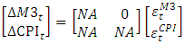
Where A is a 2*2 matrix, the vector of structural disturbances and A₀ ≠ 1. If the structural disturbances (shock to M3 and NY or shock to M₃ and CPI) are assumed orthogonal such that the estimation of VMA requires one restriction given that A is a 2*2 matrix. Thus, the structures of the two models to be estimated including their respective restrictions are given as:

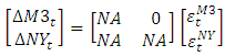(23)

(24)

The assumptions that informs restriction in equations (23) and (24) ensue to test; One, the assumption that changes in money supply influences nominal activities; and two, the Friedmanic Proposition that Inflation is a function of monetary aggregates. These restrictions can also shed some light on the validity or otherwise of the concept of long-run neutrality of money for Nigeria.

The quarterly GDP was sliced into monthly using cubic approach in Eviews 9. Thus, the data for all variables are monthly from 2009M12 to 2018M6.

4. Empirical Results

4.1. The Friedman-Meiselman Dual Criteria

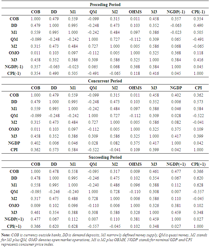
Following the methodology of Friedman-Meiselman (F-M) dual criteria, correlation analyses of components of monetary aggregates, output and prices were conducted to determine if the dual criteria holds for Nigeria during the preceding, concurrent and succeeding periods. The concurrent period considered the dataset in the same period, while output and prices were used as leading indicators of monetary aggregates for the succeeding periods and as lagged indicators in the case of the preceding periods.

The result shows that the CBN bills held by money holding sectors has a strong relationship with output relative to the other components of monetary aggregates, hence, justifying its inclusion as a component of broad monetary aggregate. Furthermore, when correlated with output, M2 monetary aggregate for all the periods did not satisfy both conditions of F-M dual criteria because its coefficients (0.068, 0.082 and 0.110) for all the periods are lower than those of its components, however, M3 monetary aggregate satisfied both conditions of the criteria given that its coefficients (0.384, 0.417 and 0.459) are higher than those of its components as presented in Table 1.

Table 1. Correlation between Changes of Components of Monetary Aggregates and Macroeconomic Variables

Similarly, the correlation between changes in M2 and prices violated both conditions of the F-M approach as its coefficients (-0.065, -0.041 and -0.045) are lower than the coefficients of its components for all the periods. However, the first and second conditions for the F-M dual criteria were satisfied for changes in M3 in relation to prices for the preceding, concurrent and succeeding periods. Consequently, the inclusion of CBN bills holdings by the money holding sectors in M2 to obtain M3 resulted in a better correlation with output and prices for all the periods. This study on M3 provides a better outcome than the study by Yaaba (2017) which concluded that the approach to monetary aggregation in Nigeria using M2 as broad money aggregate is although functionally coherent but only fairly empirically cogent.

Overall, the result confirms both the first and second conditions of the F-M dual criteria for all periods for output, thereby making M3 the appropriate definition of monetary aggregate for Nigeria. However, for prices, the result failed to confirm the first condition but satisfies the second F-M dual criteria.

The above findings revealed that M3 is the most appropriate definition of broad monetary aggregate for Nigeria given that it satisfied both functional and empirical considerations in the determination of the proper definition of broad measure of money supply. This is not surprising given the quantum of the CBN bills held by the money holding sectors.

4.2. Statistical Properties of the Data

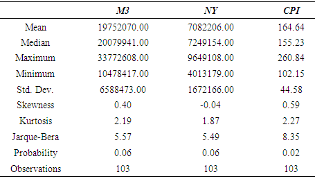
Summary Statistics

The characteristics of the variables are first explored using descriptive statistics as reported in Table 2. The table reveals that there are 103 observations per variable. While M3 and CPI are positively skewed, NY is negatively skewed. The reported Skewness coupled with the minimum Kurtosis and Jarque-Bera of 1.87 and 5.49, and maximum of 2.27 and 8.35 shows that the distribution is asymmetrical.

Table 2. Summary Statistics of the Variables used for the Estimation

Unit Root Test

The study adopted Augmented Dickey-Fuller (ADF) based on Akaike Information Criterion (AIC) and Phillips-Perron (PP) tests to determine the level of stationarity of the data. Both techniques return the variables as I(1) stationary except for NY that is neither returned I(0) nor I(1) by ADF based on AIC.

Table 3. Unit-Root Test of the Data used in the Estimation

The optimal lag length is determined based on AIC and the table is presented in the appendix as Table 4. Cursory examination of the table shows that lag two is reported as optimal by Akaike Information Criterion.

4.3. Impulse Response Functions and Variance Decomposition

4.3.1. Impulse Response Functions

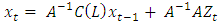
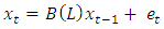
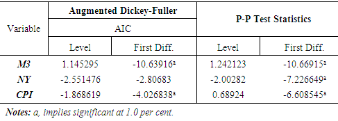
The bivariate SVAR models were run using the newly introduced higher order monetary aggregate (M3) and nominal gross domestic product and the same M3 with inflation proxy by consumer price index (CPI). In each case, the optimal lag length is determined using Akaike Information Criterion (AIC), the SVAR is run and Impulse Response Functions (IRF) and Variance Decompositions (VD) retrieved.

As common with monetary SVAR especially in relation to IRF and VD, we didn’t attach importance to Cointegration of the baseline VAR. The IRF follows analytic (asymptotic) response standard errors, using Cholesky-dof adjusted decomposition approach, while the VD is carried out using Cholesky decomposition factorization with Monte Carlo standard errors. The ordering for Cholesky is ∆M3, ∆NY for the first SVAR model and ∆M3, ∆CPI for the second model, in that order, with 100 repetitions for Monte Carlo.

Figure 1 presents the impulse responses to Cholesky one standard deviation innovations within a confidence band of two standard errors (i.e. 95 per cent confidence bands). The first column of Figure 1 reveals the reactions of M3 and NY to a positive shock on M3. The two standard deviations are represented by the two dashed lines, while the impulse response is represented by the solid lines. Close scrutiny of the first column shows that a shock to M3 leads to a highly persistent positive shock to NY. The response was strongest in the second period and began to fades gradually but never touches zero throughout the ten periods considered. This shows that a positive shock to M3 has statistically significant impact on GDP. The story however differs if we consider the second Column of the same figure. M3 is initially reluctant to respond to shock in NY but negatively and significantly responds in the second month and turn positive in the third month but dissipates rapidly to zero thereafter.

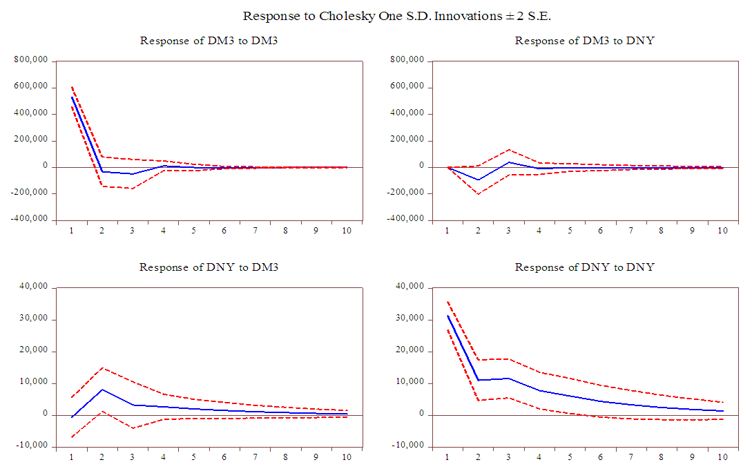Figure 1. Impulse Responses of M3 and NY to M3 Shocks

Figure 2 displays the impulse responses of M3 and CPI to shocks on M3. The lower chart of the first Column of the figure exhibits similar characteristic as the lower chart of the first Column of Figure 1. CPI responds positively to shock in M3, the shock significantly declines in the second period, but headed upward again in the third period and thereafter dissipates gradually but never touches the base. This also shows persistence in inflation in Nigeria and partially corroborates Friedmanic proposition. Although monetary aggregates determine, to a large extent, the trend of inflation in Nigeria but there are other factors. In other words, structuralist and open economy/globalist views of inflation plays some role in determining the trend of inflation in Nigeria.

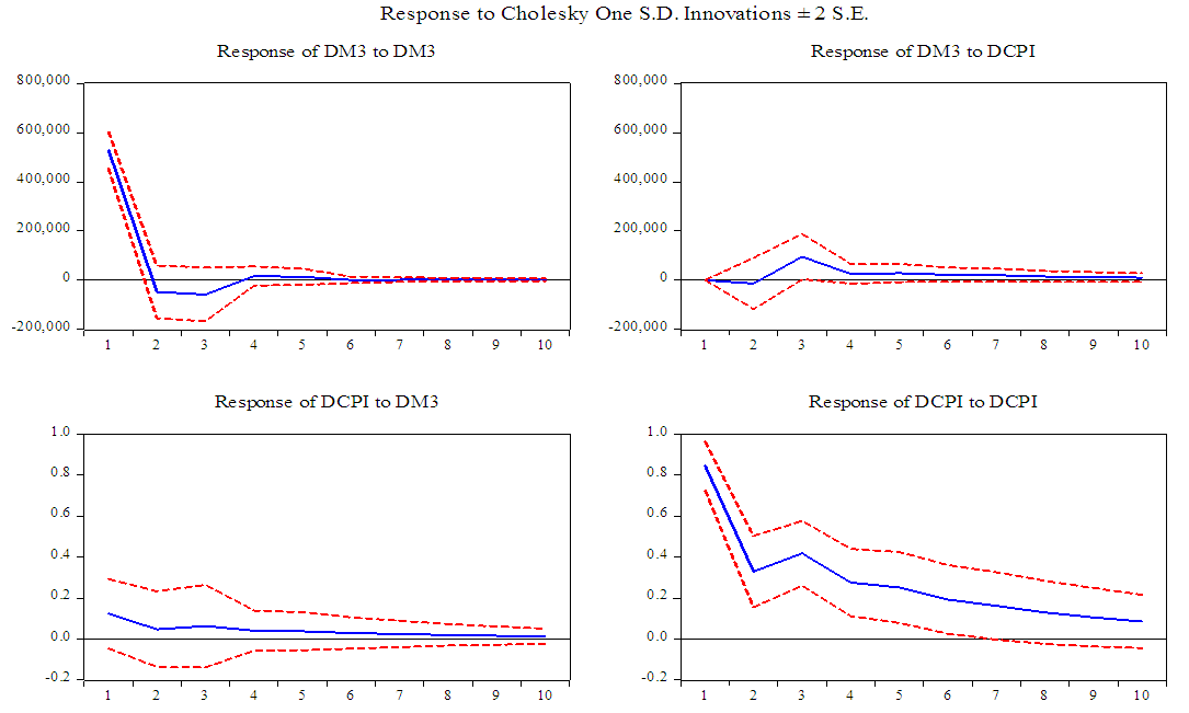Figure 2. Impulse Responses of M3 and CPI to M3 Shocks

The upper part of the second Column of the figure shows that with shocks from inflation, M3 remains neutral up to the second period when it turns slightly negative but turns significantly positive in the third period after which it dissipates gradually and slowly and flattened immediately but never touches the base throughout the period. This can be interpreted to mean that as prices react to shock on M3, so does M3 respond to shock to prices, although the magnitude of the reactions varies with prices reacting to M3 been far more on the reverse. Another distinguishing characteristic is that while the response of prices to shock in money supply is instantaneous that of M3 to shock on prices is not.

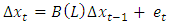
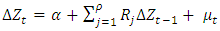
4.3.2. Variance Decompositions

Variance decomposition in VAR⁸ helps in detecting the extent of variability in the dependent variable that is lagged by its own variance. In other words, it shows the independent variable as well as its lag, that is stronger in explaining the variability in the dependent variable over the chosen period. It can therefore be said that variance decomposition assesses the degree of shocks through the relative share of variance that each of the structural shocks contributes to the total variance of each variable.

Figures 3 and 4 present Variance Decompositions of both models. Close examination of Figure 3, for instance, shows that, for the VD of M3, the GDP variance decomposition shrinks for the first two lags and increased gradually until the last lag, while monetary aggregate built-up until lag 4 when it began to shrinks until lag 9. Coincidentally, the second lag in both cases recorded the utmost growth. For the VD of the level of economic activities (GDP) depicted by the lower region of Figure 3, the first two lags of M3 inched up and began to dissipate at the fourth lag. This continues until the last lag. Conversely, the first two lags of M3 shrank and began to inch-up at the fourth lag until the last lag.

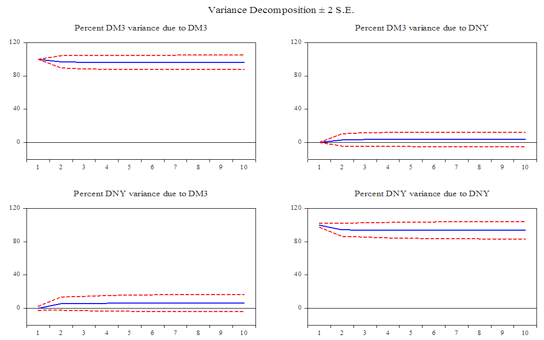Figure 3. Variance Decomposition of the SVAR Model - M3 and NY

For the second model presented as Figure 4, the VD of M3 reveals that the general price level (CPI) inched-up throughout the observed period, while that of M3 shrank throughout the period. The VD of CPI represented by the lower portion of the figure shows that only the second lag of the M3 dissipates and thereafter built-up until the end of the sample period. This is against GDP which only began to shrink at lag 3 until lag 7.

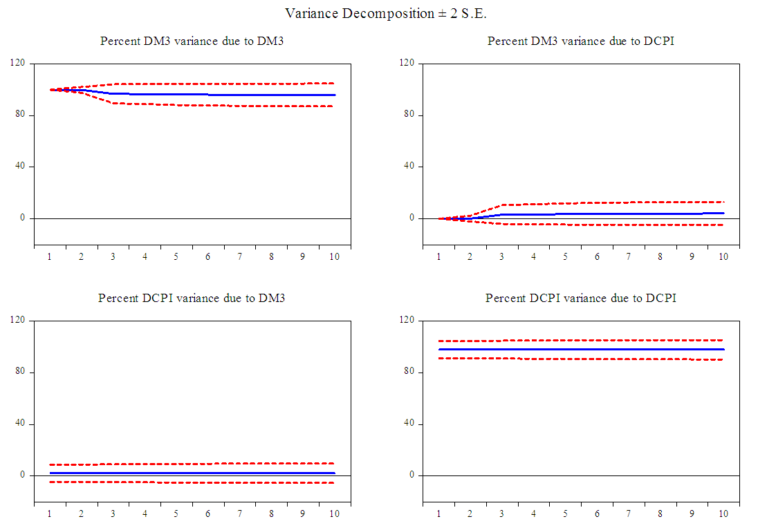Figure 4. Variance Decomposition of the SVAR Model - M3 and CPI

5. Conclusions and Policy Remarks

Developments in the Nigerian financial markets arising not only from new entries or exits of market players but also from the advent of new instruments has necessitated the introduction of a higher order monetary aggregate, M3. Banks were in the fore front of these innovations competing to dominate each other in the market share of the new products. This development necessitated realignment in the definition of monetary aggregates to ensure that stable relationship is maintained between money supply, inflation and output for the Central Bank of Nigeria to achieve its mandate of ensuring price stability conducive for economic growth. The new monetary aggregate encompasses currency outside banks, demand deposits at CBN and other private sector demand deposits at other depository corporations, quasi money and OMO Bills held by money holding sectors. In an effort to validate the new monetary aggregate, this study subjected the M3 to F-M dual criteria as well as adopted SVAR to determine its relationship with output and the general price levels.

The results of the SVAR report high persistent positive response of the level of economic activities arising from positive shock to M3 and similar, but of less magnitude, response of prices to shock in M3. Conversely, there is a reluctant response of M3 to shocks to both the level of economic activities and prices. We therefore submit that M3, in line with economic theory, contains enormous information about output and inflation in Nigeria. In other words, M3 fuels movements in both nominal output and prices in Nigeria. The results also reveal that M3 satisfies the F-M dual criteria. The study therefore, supports the adoption of the new higher order monetary aggregate (M3) as the broadest definition of money for Nigeria.

Notes

1. The views here-in expressed are solely ours and do not represent or necessarily reflects that of Central Bank of Nigeria where we work.

2. Some EU members that are non-Euro area members also comply with the concepts and definitions of the ECB

3. Nigeria recently included securities issued by DCs and held by money holding sector, which broadens the national definition of broad money, hence, the introduction of a higher order monetary aggregate, M3.

4. Non-residency is determined by an entity’s centre of predominant economic interest rather than nationality. If an entity intends to engage in business activities in a particular country for more than a year, it is considered as resident otherwise it is non-resident.

5. Money-holding sectors in Nigeria include Other financial corporations, State and local government, nonfinancial corporations, households and non-profit institutions serving households

6. ODCs deposits at CBN includes required reserves, current accounts and other special deposits

7. Pedroni (2013) for detail.

8. And by extension SVAR