1. Introduction

It has become crucial that price stability is the principal objective for the conduct of central banks’ monetary policy. Changes of inflation dynamics, such as the level of inflation rate and inflation expectations, will have significant impact on monetary stability-one of the main monetary policy goals.

The empirical literature on the postwar US inflation has documented that the inflation process has slow responses to shocks and tends to approach its mean level slowly rather than instantly, which has become persistent since World War II (Marques, 2004; Williams, 2006). Yet the degree of inflation persistence and its variability have remained disputable.

Studies show that US inflation persistence was very high from 1965 to the early 1980s (Brainard and Perry, 2000; Taylor, 2000; Kim et al., 2001; and Cogley and Sargent, 2001 and many others). Fuhrer and Moore (1995) documented extremely high inflation persistence during the postwar period, approaching that of a random walk process. Also Pivetta and Reis (2007) find that US inflation is best described as high and time invariant since 1965. This implies that the best forecast of next year’s inflation is the most recently observed inflation rate, and it is unlikely to converge to its mean after a shock.

Whereas evidence of low inflation persistence in the 1947-1959 period and the 1960s has been found by Barsky (1987). Also low inflation persistence during the Volcker-Greenspan era is reported by among others, Brainard and Perry (2000), Taylor (2000), Kim et al. (2001), Cogley and Sargent (2001), Levin and Piger (2003) and Williams (2006). These authors favour the view that inflation tends to return to its mean after a quick adjusting shift following a shock, suggesting that therefore inflation is less persistent.

If changes in inflation persistence are observed, could they be associated with inflation rate, or with inflation volatility, or with a mixture of the two? Following a microeconomic approach, Taylor (2000) finds that inflation level is positively correlated with inflation persistence. In Taylor’s study, he examines this correlation through a microeconomic model. Similarly, Cogley and Sargent (2001) point to the combination of high inflation volatility and persistence in the late 1960s and 1970s, and lower persistence and volatility in the 1980s and 1990s. Therefore, this leads to conjecture that some links may exist between inflation, inflation persistence and uncertainties.

Meanwhile Erceg and Levin (2003) pointed out that inflation persistence can be generated when a central bank is lack of credibility– the extent to which the public believes that policies announced by the monetary authorities will be carried out (McCallum, 1985). As Fellner (1976) introduced the credibility hypothesis, central banks with full credibilitycould achieve monetary goals successfully without "causing major hardship even during the transition phase" (Fellner, 1976, p. 116).

Previous empirical studies on assessing credibility have been through the dynamics of macroeconomic variables. For example, Hardouvelis and Barnhart (1989) modelled the response of commodity prices to weekly M1 announcements, taking the difference between the Fed’s inflation forecast and the expectation of the public. Their research nonetheless under the assumption that the Fed had a single monetary policy goal. Actually the Fed holds a dual goal: sustainable output and employment and price stability. Moreover Croushore and Koot (1994) consider the difference between the Fed’s forecast and the actual inflation, while Tanuwidjaja and Choy (2006) calculate the gap between the inflation target and public expectations respectively. This method requires making use of monetary authorities’ inflation target or forecast – a requirement which cannot always be adequately met.

Given the limitations of the above approaches, this paper developes a modified and reduced form of accelerationist Phillips curve¹ (PC). This type of PC is capable of examining the postwar US inflation-unemployment trade-offs², considering the while capturing the degree of inflation persistence, and therefore testing for the credibility hypothesis to fill in the gap in the literature. When a flattened Phillips curve is estimated, it shows that the link between inflation and other macroeconomic variables is weak. For example, lowering inflation will not result in a severe increase in unemployment or reduction in output. For example, Cagan and Fellner (1983) demonstrated that credibility played an important role in the shifts in responses to policy measures for the US cycles from 1953-1981.

Section two discusses the credibility hypothesis, disinflation cost and the dispute between them. Section three describes the measures of inflation persistence and expectations, the accelerationist Phillips curve and the model applied in this paper. Section four proceeds to estimate the parameters and presents the results, which are discussed in section five. Finally section six concludes.

2. The Credibility Hypothesis, Disinflation Cost and Solutions

The credibility hypothesis seems to fit well in interpreting the US economic performance for most of the postwar episodes (McCallum, 1984; Plosser, 2007). A recession occurred in 1961, lasting for ten months. Then, an expansion followed spanning 106 months. During this period, the Fed successfully maintained inflation at a low and stable level with growth in employment (average unemployment rate of 4.96%). This is accordingly recorded as a period of economic prosperity with growth and stability (Schumann, 2001).

When a recession started in November 1970, the spread of economic prosperity was halted. Inflation was accelerated to be persistently high. Average monthly inflation rates peaked at nearly 1% in 1974, while unemployment rose to a peak of 9% in May 1975. One of the main causes of this stagflation period was the oil price, which sharply increased in 1973-1974 and 1979. The failure to maintain price stability damaged the Fed’s credibility, consequently inducing long lags between the introduction of more aggressive counter-inflationary policies and actual falls in the inflation rate (Yellen, 2006). It was not until the second recession ended in November 1982 that inflation began to decline. During the period of January1984-December 1989, monthly inflation and employment rates averaged at 0.36% and 6.44% respectively, signifying that the US re-entered into a period of low inflation environment and resumed credibility of the Fed (Belton Jr. and Cebula, 1998).

Further, the Fed made an announcement of Zero-Inflation Resolution (Greenspan, 1989) to confirm its determination to maintain price stability in October 1989, which was succeeded the longest economic expansion of any ten-year period since the end of WWII. Inflation and unemployment rates, averaging 0.22% and 5.76% respectively, as well as the policy lags had been markedly reduced.

The US experience of low inflation together with strikingly high unemployment in the early 1980s gave rise to a vigorous debate. First, Perry (1983) pointed out that disinflation was followed by the recession at great loss, during which unemployment arose to more than 10% in the fourth quarter of 1982, which was worse than the severe 1975 recession. In particular, B. Friedman (1984) used annual price inflation, real growth and unemployment to calculate the disinflation cost in terms of "the cumulative excess of the unemployment rate" estimated at 2.7%, 6.4% and 10.1% for 1980, 1982 and 1983 respectively (p. 385). This is around the range of the conventional prediction by Okun (1978), who estimated the cost of disinflation by inspecting six accelerationist Phillips curves and indicated that "for an extra percentage point of unemployment maintained for a year, the estimated reduction in the ultimate inflation rate at equilibrium unemployment ranges between one-sixth and one-half of 1 percentage point, with an average estimate of 0.3." (p. 348). B. Friedman (1984) concluded that the costs of disinflation were as previously predicted, and the introduction of money supply targets had not reduced those costs.

To solve this puzzle, firstly NAIRU is a crucial element. Assuming a NAIRU of 6.5% with a 5% drop in inflation, Fischer (1984) worked on the same data and found the cost was below the range quoted by Okun, implying that the switch of monetary policy effectively reduced the disinflation cost. This NAIRU hypothesis was later proved by Gordon (1997). His finding suggested a time-varying NAIRU of the US, which climbed over 6.0% in the early 1980s.

Secondly, there has been controversy over the extent of the Fed’s credibility in the early 1980s. Clarida and B. Friedman (1983), B. Friedman (1983, 1984), Perry (1983), and Croushore and Koot (1994) considered the Fed credible. The opposite was shared by, among others, Hardouvelis and Barnhart (1989), and Belton Jr. and Cebula (1998). As discussed in the introduction, credibility depends on inflation expectations. Having a glimpse of various expectations of the public for 1980-1983, both Michigan Surveys and Survey of Professional Forecasters show an average inflation over 7%, which is higher even than the 1970s average of around 6.5%. Although the Livingston Survey shows a lower expected mean for 1980-1983 at 3.1%, it is still higher than that of its survey in the previous decade. This rough evaluation reflects a negative attitude that the public did not seem to believe in the Fed’s disinflation policy completely and consequently disinflation corresponded to a great cost. In his speech, Ferguson (2005) noted that "this credibility is hard won, however, and can be easily lost".

Thirdly, the controversy about credibility is due to the imperfect knowledge of policy efforts (Fellner, 1982), which Friedman (1972, p. 17) explained earlier: "the public at large has been led to expect standards of performance that as economists we do not know how to achieve". Besides, Fellner (1982, p. 90) suggested that "one needs to be very selective in constructing one’s sample period to find that this rival hypothesis does about equally as well as the credibility hypothesis".

3. Empirical Approaches

3.1. Measuring Inflation Expectations

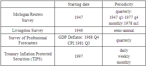
There exist several surveys measuring inflation expectations, such as the Reuters/University of Michigan Surveys of Consumers, Livingston Survey and Survey of Professional Forecasters, and the measure derived from inflation-indexed bonds – Treasury Inflation Protected Securities (TIPS). These surveys represent the expectations of economists, consumers and financial market participants on inflation, with the range and periodicity shown in table 1.

Table 1. Surveys of inflation expectations and inflation-indexed bonds

On the other hand, expectations can also be formed from a model. For example, the FRB/US model assumes that the public’s expectations are depended on the historical relationship between inflation and other economic variables (Brayton et al., 1996).

This paper examines monthly inflation data with a long range, thus measures based on surveys and derived from the bond market are unable to represent inflation expectations. For this reason, the lags of inflation are used, which also contribute to overcome the not perfectly rational expectations (Roberts 1998, Gali and Gertle 1999, and Adam and Padula 2003).

3.2. Modelling Inflation Persistence

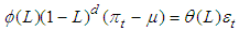
Batini and Nelson (2001, p.383) identify three different types of inflation persistence: "positive serial correlation in inflation", "lags between systematic monetary policy actions and their (peak) effect on inflation", and "lagged responses of inflation to non-systematic policy action (i.e. policy shocks)". While Willis (2003, p.7) considers inflation persistence as "the speed with which inflation returns to baseline after a shock". The latter definition is the most widely accepted or modified. In this paper, we use the Willis’ definition of inflation persistence, which concerns the speed of the responses of inflation to shock. As Willis (2003) noted " Such shifts in the behavior or dynamics of inflation would necessitate changes in the economic relationships used by policymakers and economists to assess current conditions, forecast key economic indicators, and determine the implications of policy changes for future economic activity." (p. 7)

Furthermore, the reaction of a series to shocks can be categorized into three types: (i) the persistence decays at an exponential rate (short memory), (ii) it decreases at a hyperbolic rate (long memory), or (iii) infinitely (perfect memory). The three categories corresponded to different degrees of integration of a time series. A process with short memory is stationary (integrated with degree zero), a series with perfect memory is integrated with degree 1 and a series with long memory is integrated to a fraction. To characterise the significant autocorrelation between observations of a time series dynamic, a univariate autoregressive fractionally integrated moving average (ARFIMA) process, developed by Granger (1980) and Granger and Joyeux (1980), is possible to capture inflation persistence, which is expressed as follows:

(1)

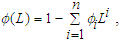
where stands for inflation, is the intercept, and is the disturbance term, which is serially uncorrelated and follows a Gaussian distribution. L is the lag operator³, 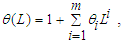and both and roots lie outside the unit circle. Here accounts for the long memory and is defined as:

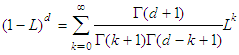With denoting the Gamma function. The parameter of d, lying between zero and unity, measures the speed of that inflation’s convergence to equilibrium after a shock to an I(d) process.

Baillie et al. (1996) explain the general properties of an ARFIMA process. When d=0, the series is an I(0) process with short-run behavior, in which the effects of shocks fade at an exponential rate of decay; that is, the series quickly regains its equilibrium. In the case of an I(1) process (when d=1), following a shock, the series does not revert to its mean and the persistence of shocks is infinite. Between the distinctive I(0) and I(1), an I(d) process with long-run dependence, when 0<d<1, in which persistence dies out hyperbolically. In this case, the series takes a considerable time to reach mean reversion after shocks. Specifically, when d>0.5, the series is non-staionary. (Mills, 1999, p.115)

3.3. Accelerationist Phillips Curve

William Phillips (1958) describes an inverse relationship between money wage changes and unemployment in the British economy over the period of 1861-1957. Similarly, Paul Samuelson and Robert Solow’s (1960) work explicitly shows that this link between inflation and unemployment based on both UK and US data, that is, when inflation rate is high, unemployment rate is low. Phillips’ (1958) results also show that there is a permanently stable relationship between inflation and unemployment. While the traditional Phillips curve fails to capture the long-term trade-off between the US inflation and unemployment rates (see, for example, Samuelson and Solow, 1960).

In the 1960s, Friedman (1977) and Phelps (1994) developed the hypothesis that in the long-run there is a natural rate of unemployment or NAIRU (the acronym stands for ‘non-accelerating inflation rate of unemployment’), defined as "the current equilibrium steady-state rate, given the current capital stock and any other variables. In theory, then, the equilibrium path of the unemployment rate is driven by a natural rate that is a variable of the system rather than a constant or a forcing function of time" (p. 1). At that natural rate, inflation could be at any absolute level (although the rate itself will be stable). This hypothesis explains that the Phillips curve is a short-term relation rather than a long-term one.

In particular, Gordon (1997) developed a ‘Triangle Model’ to characterise short-run inflationary behaviour. With three determinants – demand for inflation (due to a fall in unemployment or a rise in output), supply shock of inflation (such as oil shocks), and inflation inertia.

3.4. The Model

Based on Gordon’s triangle model, the general model in this paper is written as:

(2)

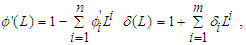
where is a variable capturing supply shocks, 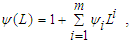and all and roots lie outside the unit circle. is unemployment and is a time series of NAIRU. To obtain the series of , a Hodrick-Prescott filter (Hodrick and Prescott, 1997) is used to smoothen the actual unemployment process, which has been applied in large literature (for example, Ball and Mankiw, 2002).

The slope coefficient is negative, which shows the trade-off between inflation and unemployment. shows the impact of supply shocks on inflation. When higher credibility is achieved, the estimated values of and are expected to be lower, reflecting that inflation has a weak link with unemployment as well as with supply shocks.

The inflation rates in equation 2, unlike the traditional Phillips curve, are modelled as an ARFIMA process. In addition to proxy for inflation expectations, this model is a flexible representation of the degree of inflation persistence. If the estimated value of d is very close to unity, the restriction of unit root then will be imposed to estimate again. Indeed, the postwar US inflation process does not follow a random walk entirely all the time as shown by the unit root tests shown in table 2. Hence, the model of equation 2 is capable of linking expectations and inflation persistence, and testing for the credibility hypothesis.

4. Empirical Results

4.1. The Data

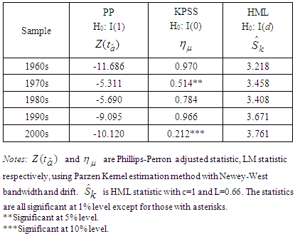
The measure of inflation in this paper is the natural log difference of core CPI (consumer price index for all urban consumers, all items less food and energy), that is. Unemployment is the civilian unemployment rate and supply shocks are the relative spot price of the West Texas Intermediate (WTI) blend of crude oil. This study employs monthly data corresponding to the postwar period (1960:01-2009:12). Core CPI and unemployment are seasonally adjusted taken from the U.S. Bureau of Labor Statistics and the oil price is obtained from Dow Jones & Company. In this connexion, the path of oil prices relative to core inflation reflects the stance of the Fed’s monetary policy in the short-run, responding to incoming temporary supply shocks (Mishkin, 2007a).

As Fellner (1982, p. 91) mentioned: "it would be unwise to quantify nominal demand goals for periods shorter than a cycle", since "highly imperfect knowledge of these relations⁴ sets limits to successful countercyclical demand policy efforts". Therefore, for the purpose of examining the Fed’s key short-run objective of stabilizing the economy, the data used in this paper are divided into five subsamples since 1960s⁵ according to the business cycles defined by NBER. In this way, the chosen procedure acts "smoothing out the peaks and valleys in output and employment around their long-run growth path". (see U.S. Monetary policy: An Introduction, 2004, p. 5)⁶

To identify such a stylised fact of the persistence of inflation dynamics, several unit root tests are employed. The Phillips-Perron (PP) test is used for the null hypothesis of a unit root against the alternative of stationarity. In contrast, the null hypothesis in the Kwiatkowski, Phillips, Schmidt, and Shin (KPSS) test is that the series is stationary, that is I(0), which is based on the statistic⁷ 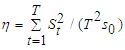. Unlike the two threshold tests, the HML (Harris et al., 2008) test is for the null hypothesis of short memory against long memory alternatives, that is the test of I(0) against I(d).

Table 2 reports three unit root tests, PP, KPSS and the HML tests as discussed above for postwar inflation series. The PP test statistics for three subsamples (1960s, 1990s and 2000s) are significant at 1% level, while the KPSS statistics imply that the tests reject the null of stationarity at 1% level, except for 1970s and 2000s subsamples at 5% and 10% level respectively. This indicates that it is not for all subsamples of US inflation that inflation follows a random walk process. Finally HML tests reject the null of inflation following an I(0) process for all the subperiods. Our results suggest, in general, that the inflation process is best described as I(d), rather than I(1) or I(0), and that an ARFIMA is the proper methodology to assess the integrability of this series.

Table 2. Unit root tests for inflation

4.2. Estimates

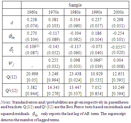
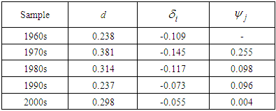
Using ordinary least squares (OLS), equation 2 is estimated by minimizing the sum of the squared residuals. The Phillips curve OLS estimation has been widely used in the literature, for example, Williams (2006), Puzon (2009).⁸ Table 3 presents the Phillips curve estimates of inflation-unemployment. The estimated values of d are 0.24, 0.38, 0.31, 0.24 and 0.30 for the subsamples of 1960s, 1970s, 1980s, 1990s and 2000s respectively. They are all between zero and 0.5 and significantly distant from 0 or 1 with small standard error, implying that the each subsample of the inflation process exhibits a long memory feature.

Table 3. Inflation-Unemployment accelerationist Phillips curve estimation results

The estimation results of slope coefficient δ are all negative, demonstrating the Phillips curve in each individual decade. Notably, the slope coefficient is not immutable, but has changed as persistence varies over decades. When inflation was very persistent in 1970s, the Phillips curve was steep, that is a unit decrease of unemployment deviating from NAIRU was followed by 15% increase in inflation. As persistence has declined over last two decades, the Phillips curve has had a flattening tendency.

On the other hand, the impact of the oil price on inflation in the 1970s was estimated strong: a unit rise of oil price resulted in a 26% increase in inflation. By contrast, during the other decades with a flatter Phillips curve and lower degree of persistence, the oil price did not have a significant effect on inflation. Specifically, during the 1960s, inflation was quite stable, and did not respond to the oil price at all. As Blanchard and Gali (2007, p. 65) concluded, "the effects of oil price shocks have changed over time, with steadily smaller effects on prices and wages, as well as on output and employment", which may be caused by "the increased credibility of monetary policy".

The estimates shown in table 4 provide the results of testing the credibility hypothesis. In 1960s, inflation rates were stable, not influenced by oil price and weakly related to unemployment. This indicates that the Fed was credible. However, in 1970s, the Phillips curve was steep and the inflation process was affected by oil price strongly, implying that the public had little faith in the Fed. As the Phillips curve has appeared to be flattening since 1980s, as well as inflation becoming less responsive to the oil price, it seems that the Fed has regained its credibility.

Table 4. Statistics for testing credibility hypothesis

5. Discussion

By the definition of credibility in this paper that public believes announced disinflationary policy have actually been carried out, it is essential to check back the Fed’s track records of credibility.

From 1957 through the end of 1960s, two recessions occurred (1958 and 1961) eight months and ten months respectively. When the second recession ended in February 1961, there was a boom spanning 106 months. During this period, the US inflation was recorded as a low and stable level– the monthly inflation averaged around 0.21%. With growth in employment (average unemployment rate of 4.96%), this was a period of economic prosperity (Schumann, 2001). Having maintained price stability, as a result the Fed gained credibility.

When the recession started in November 1970, the spread of economic prosperity was halted. Inflation was accelerated to be persistently high, for example average monthly inflation rates peaked at nearly 1% in 1974. One of the main causes of this stagflation was the oil price, which was sharply increased in 1973-1974 and 1979. Worse yet, the unemployment rose to more than 6% and peaked at 9% in May 1975. The failure of maintaining price stability resulted in that the Fed’s commitment was not believed, consequently inducing long lags of policy on lowering inflation.

After enduring stagflation in 1970s, the Fed announced a major policy shift by tightening the money supply to lower inflation in November 1979. While it was followed by a short recession lasting six months. Monthly inflation and unemployment rates kept high averaging 0.9% and 7.25% respectively. Until the second recession ended in November 1982, inflation began to fall down as monthly inflation rates averaging 0.36% for the period of January1983-December 1989, which symbolized that the US ushered in a low inflation economic environment as well as the resumed credibility of the Fed.

In October 1989, the Fed made an announcement of Zero-Inflation Resolution (Greenspan, 1989) to confirm its determination to maintain price stability, which brought the longest economic expansion of ten years since the end of WWII. Inflation and unemployment rates, averaging 0.22% and 5.76% respectively, as well as the policy lags had been reduced. Undoubtedly, the Fed had regained credibility, which succeeded in the 2000s.

These track records of the Fed’s credibility have been exactly displayed by the results of estimating equation 2, which reveal that credibility is negatively related to persistence indeed. For the decades of 1970s and 1980s with higher persistence, the public had little faith in the Fed’s commitment to price stability. When inflation was less persistent in 1960s, 1990s and 2000s, the Fed gained credibility. A disinflationary policy is credible, as long as it has been implemented to achieve low inflation without much delay, and vice versa. Therefore, the degree of inflation persistence herein, as a reliable variable, indicates the evolvement of the Fed’s credibility.

6. Conclusions

This paper has assessed the Fed’s credibility by testing the credibility hypothesis for each decade during postwar period. A modified and reduced form of accelerationist Phillips curve has been used to analyse inflation-unemployment trade-off, which forms inflation expectations in an ARFIMA procedure and therefore captures the property of inflation persistence.

The results of these Phillips curve estimates have shown a steep Phillips curve for the 1970s and 1980s, and a flattened Phillips curve for the 1960s, 1990s and 2000s. As for the supply shocks, before the first oil shock, inflation was quite stable and did not respond to oil price at all in 1960s. When oil shocks occurred twice in 1970s, oil prices had a powerful impact on inflation, but from the 1980s onwards the oil price ceased to have a strong influence on the overall price level. More importantly, the positive relation between the degree of inflation persistence and the absolute value of the slope coefficient of inflation-unemployment has been revealed. When inflation was relatively less persistent in 1960s, 1990s and 2000s, the Phillips curve was flattened implying gains in Fed credibility.

A disinflationary policy is credible, as long as it is implemented to lower inflation without much delay, and vice versa. The degree of persistence reflects the velocity of inflation responding to a change in monetary policy. However, other measures of credibility which do not account for persistence may not be adequate – in particular, the calculation of disinflation cost in the disputes of the early 1980s. As a reliable variable, inflation persistence reveals the Fed’s credibility. Credibility enables the Fed to adjust the public’s inflation expectations and so to attain its disinflation goal more rapidly. In turn, a decrease in inflation persistence signifies that credibility has been obtained.

The results of estimating the Phillips curve have shown that inflation is relatively stable despite a significant impact of the oil price shocks in 1970s. More importantly, it has revealed a positive relation between the degree of inflation persistence and the absolute value of the slope coefficient of inflation-unemployment. Thus an important conclusion can be drawn: the credibility of a disinflationary policy hinges on its expeditious implementation, and vice versa. The degree of persistence reflects the speed with which inflation responds to a change in monetary policy, and hence reveals the dynamic of the Fed’s credibility. Findings herein imply higher degrees of inflation persistence with less credibility in the 1970s and 1980s, and lower degrees of inflation persistence with more credibility in the 1960s, 1990s and 2000s. Future studies could consider the volatilities of inflation dynamics as well as other macroeconomic variable for a deeper insight into series. For instance, a bivariate or multivariate model can be conducted with consideration of volatilities, which may provide some other important information for the monetary policy credibility.

ACKNOWLEDGEMENTS

I would like to thank seminar participants for their helpful comments and suggestions. The usual caveat applies.

Notes

1. See Fisher (1926) and Phillips (1958).

2. See Cagan and Fellner (1983), Ball, Mankiw and Romer (1988), Kahn and Weiner (1990), Lalonde (2005), Karanassou and Sala (2008).

3.

4. These relations refer to "the relevant serial correlation among data, including the lags involved in these" and " the lags involved in influencing the real variables by policy action" (Fellner, 1982, p. 91).

5. The subsample of 2000s is from January 2000 to December 2009.

6. It is available at http: // www.frbsf.org / publications / federalreserve/ monetary.

7. and is an estimator of the residual spectrum at frequency zero.

8. Some other estimation methodologies are also used in the literature such as generalized method of moments (GMM), Instrumental Variables Two-stage Least Squares Regression. As Singh et al. (2011) explain in their recent work, OLS method could be problematic, since the variables in the model “are dated to the same time” (p. 256). While this study considers different lags of each variable, therefore OLS estimation is appropriate to be applied for estimating the Phillips curve in this paper.