1. Introduction

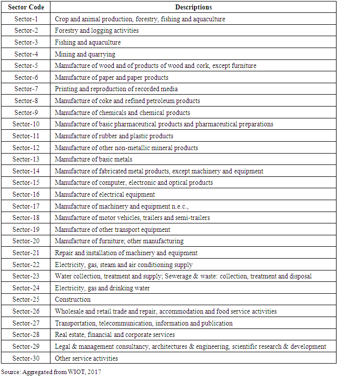
The USA economic activities create multipliers to other-countries economy. It multiplies output that were initially created by the USA economy, directly, indirectly and induced to other-countries, as well as to other-sectors. In macroeconomics, a multiplier is a factor of proportionality that measures how much an endogenous variable changes in response to a change in some exogenous variable (see among others: Dornbusch & Stanley, 1994; McConnell, et., al, 2011; Pindyck & Rubinfeld, 2012). In monetary microeconomics and banking, the money multiplier measures how much the money supply increases in response to a change in the monetary base (see among others: Krugman & Wells 2009; Mankiw, 2008). Multipliers can be calculated to analyze the effects of fiscal policy, or other exogenous changes in spending, on aggregate output. Other types of fiscal multipliers can also be calculated, like multipliers that describe the effects of changing taxes.

Literature on the calculation of Keynesian multipliers traces back to Richard Kahn’s (1931) description of an employment multiplier for government expenditure during a period of high unemployment. At this early stage, Kahn’s calculations recognize the importance of supply constraints and possible increases in the general price level resulting from additional spending in the national economy (Ahiakpor, 2000). Hall (2009) discusses the way that behavioral assumptions about employment and spending affect econometrically estimated Keynesian multipliers.

The literature on the calculation of I-O multipliers traces back to Leontief (1951), who developed a set of national-level multipliers that could be used to estimate the economy-wide effect that an initial change in final demand has on an economy. Isard (1951) then applied input-output analysis to a regional economy. The first attempt to create regional multipliers by adjusting national data with regional data was by Moore & Peterson (1955) for the state of Utah. In a parallel development, Tiebout (1956) specified a model of regional economic growth that focuses on regional exports. His economic base multipliers are based on a model that separates production sold to consumers from outside the region to production sold to consumers in the region. The magnitude of this multiplier is based on the regional supply chain and local consumer spending.

In a survey of input-output and economic base multipliers, Richardson (1985) notes the difficulty inherent in specifying the local share of spending. He notes the growth of survey-based regional input-output models in the 1960s and 1970s that allowed for more accurate estimation of local spending, though at a large cost in terms of resources. To bridge the gap between resource intensive survey-based multipliers and “off-the-shelf” multipliers, Beemiller (1990) of the BEA describes the use of primary data to improve the accuracy of regional multipliers. The literature on the use and misuse of regional multipliers and models is extensive. Coughlin & Mandelbaum (1991) provide an accessible introduction to regional I-O multipliers. They note that key limitations of regional I-O multipliers include the accuracy of leakage measures, the emphasis on short-term effects, the absence of supply constraints, and the inability to fully capture interregional feedback effects.

Grady & Muller (1988) argued that regional I-O models that include household spending should not be used and argue that cost-benefit analysis is the most appropriate tool for analyzing the benefits of particular programs. Mills (1993) noted the lack of budget constraints for governments and no role for government debt in regional IO models. As a result, in less than careful hands, regional I-O models can be interpreted to over-estimate the economic benefit of government spending projects. Hughes (2003) discussed the limitations of the application of multipliers and provides a checklist to consider when conducting regional impact studies. Harris (1997) discussed the application of regional multipliers in the context of tourism impact studies, one area where the multipliers are commonly misused. Siegfried, et al (2006) discussed the application of regional multipliers in the context of college and university impact studies, another area where the multipliers are commonly misused. Input-output analysis, also known as the inter-industry analysis, is the name given to an analytical work conducted by Leontief in the late 1930's. The fundamental purpose of the input-output framework is to analyze the interdependence of industries in an economy through market-based transactions. Input-output analysis can provide important and timely information on the interrelationships in a regional economy and the impacts of changes on that economy.

The notion of multipliers rests upon the difference between the initial effect of an exogenous change (final demand) and the total effects of a change. Direct effects measure the response for a given industry given a change in final demand for that same industry. Indirect effects represent the response by all local industries from a change in final demand for a specific industry. Induced effects represent the response by all local industries caused by increased (decreased) expenditures of new household income and inter-institutional transfers generated (lost) from the direct and indirect effects of the change in final demand for a specific industry. Total effects are the sum of direct, indirect, and induced effects.

The objective of this paper is to calculates, presents and discusses on sectoral and spatial multipliers in the USA economy using 6-country-30sector input-output tables for the year 2000, 2005, 2010 and 2014 processed from World Input-Output Tables.

2. Methodology

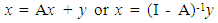
An input-output table records the “flows of products from each industrial sector considered as a producer to each of the sectors considered as consumers” (Miller & Blair, 1985). It is an “excellent descriptive device” and a powerful analytical technique (Jensen et.al, 1979). In the production process, each of these industries uses products that were produced by other industries and produces outputs that will be consumed by final users (for private consumption, government consumption, investment and exports) and also by other industries, as inputs for intermediate consumption (Oosterhaven & Stelder, 2007; Timmer, et al (2015).

The columns provide information on the input composition of the total supply of each product j (X_j), this is comprised by the national production and also by imported products. The value of domestic production consists of intermediate consumption of several industrial inputs i plus value added. The inter-industry transactions table is a nuclear part of this table, in the sense that it provides a detailed portrait of how the different economic activities are interrelated. Since, in this table, intermediate consumption is of the total-flow type, this implies that true technological relationships are being considered. In fact, each column of the intermediate consumption table describes the total amount of each input i consumed in the production of output j, regardless of the geographical origin of that input.

The input-output interconnections can be translated analytically into accounting identities. On the demand perspective, if Z_ij denote the intermediate use of product i by industry j and y_i denote the final use of product i, we may write, to each of the n products:

(1)

On the supply side, we know that:

(2)

in which w_j stands for value added in the production of j and m_j for total imports of product j. Of course, it is required that, for i = j, x_i = x_j, i.e., for one specific product, the total output obtained in the use or demand perspective must equal the total output achieved by the supply perspective. These two equations can be easily related to the National Accounts’ identities. In general term, equation (1) can be written as:

(3)

Inter-Country Input-Output Table of the USA for the year of 2000, 2005, 2010 and 2014 are available from World Input Output Data Base (Timmer et al, 2016; 2015). Calculation of total and disaggregated multipliers, sector-specific multipliers and country-specific multipliers following West (1990) and modified formula of DiPasquale & Polenske (1980). West (1990) defined the major categories of response as: initial, first-round, industrial-support, consumption-induced, total and flow-on effects. Total effect is calculated as summation of initial, direct-effect (first-round), indirect-effect (industrial-support) and consumption induced effect (as matrix is closed to house-hold row and column, which was not calculated in this study). Flow-on effect is defined as the different between total and initial effects. 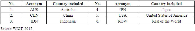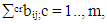Modified from DiPasquale & Polenske (1980), sector-specific multipliers of output is calculated as and country-specific multipliers of output is calculate as 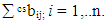Note that c and r are the m origin and destination countries, i and j are the n producing and purchasing sectors, ^crb_ij is the element of inverse of Leontief matrix, m is the number of country and n is the number of sectors. Sector classifications and Country abbreviations are available in Appendix 1 and Appendix 2.

3. Results and Discussions

3.1. Total Multipliers

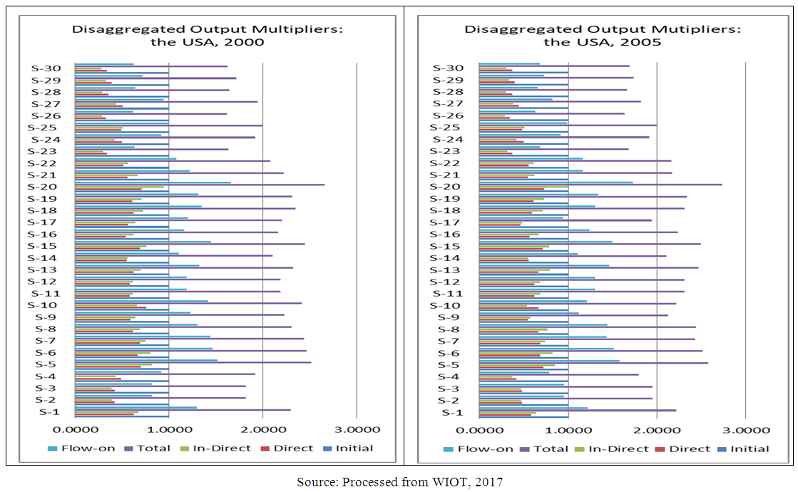
Figure 1 presents disaggregated output multipliers: direct, indirect, and total effects of output created initially in the USA economy for the year of 2000 and 2005. In the year of 2000, average national output multiplier was 2.1172; meaning that output flow-on effect was 1.1172 as initial effect was 1.0000. Direct effects of increasing final demand by 1.000 unit would be 0.5453 and indirect effect would increase by 0.5719 resulting total output multiplier of 2.1172. Please note that the flow-on effect is the summation of direct and indirect effects; it is the different between total effect and initial effect. The highest total output multiplier was in Sector-20 (2.6546) and the lowest was in Sector-26 (1.6121). In this year, there were 19 sectors in which total output multipliers more than 2; meaning that flow-on effects were higher than initial effects. These sectors were: Sector-1 (2.2964), Sector-5 (2.5157), Sector-6 (2.4673, Sector-7 (2.4417), Sector-8 (2.3042), Sector-9 (2.2281), Sector-10 (2.4105), Sector-11 (2.1889), Sector-12 (2.1891), Sector-13 (2.3221), Sector-14 (2.1049), Sector-15 (2.4459), Sector-16 (2.1616), Sector-17 (2.2025), Sector-18 (2.3496), Sector-19 (2.3147), Sector-20 (2.6546), Sector-21 (2.2165), and Sector-22 (2.0764).

Figure 1. Disaggregated Output Multipliers in the USA Economy: 2000 and 2005

In the year of 2005, average national output multiplier was 2.1305; meaning that output flow-on effect was 1.1305 as initial effect was 1.0000. Direct effects of increasing final demand by 1.000 unit would be 0.5496 and indirect effect would increase by 0.5809 resulting total output multiplier of 2.1305. The highest total output multiplier was in Sector-20 (2.7298) and the lowest was in Sector-26 (1.6323). In this year, there were 18 sectors in which total output multipliers more than 2; meaning that flow-on effects were higher than initial effects. These sectors were: Sector-1 (2.2214), Sector-5 (2.5810), Sector-6 (2.5122), Sector-7 (2.4316), Sector-8 (2.4389), Sector-9 (2.1210), Sector-10 (2.2142), Sector-11 (2.3055), Sector-12 (2.3055), Sector-13 (2.4640), Sector-14 (2.1077), Sector-15 (2.4954), Sector-16 (2.2383), Sector-18 (2.3075), Sector-19 (2.3408), Sector-20 (2.7298), Sector-21 (2.1703), and Sector-22 (2.1633).

Figure 2 presents disaggregated output multipliers: direct, indirect, and total effects of output created initially in the USA economy for the year of 2010 and 2014. In the year of 2010, average national output multiplier was 2.0573; meaning that output flow-on effect was 1.0573 as initial effect was 1.0000. Direct effects of increasing final demand by 1.000 unit would be 0.5197 and indirect effect would increase by 0.5376 resulting total output multiplier of 2.0573. In this year, there were 18 sectors in which total output multipliers more than 2; meaning that flow-on effects were higher than initial effects. The highest total output multiplier was in Sector-20 (2.8554) and the lowest was in Sector-4 (1.5231). These sectors were: Sector-1 (2.2409), Sector-5 (2.5386), Sector-6 (2.2728), Sector-7 (2.3630), Sector-8 (2.4198), Sector-9 (2.0727), Sector-10 (2.3067), Sector-11 (2.0947), Sector-12 (2.0947), Sector-13 (2.3912), Sector-14 (2.1600), Sector-15 (2.6893), Sector-16 (2.3200), Sector-18 (2.1758), Sector-19 (2.3445), Sector-20 (2.8554), Sector-21 (2.1518 ), and Sector-22 (2.0565).

Figure 2. Disaggregated Output Multipliers in the USA Economy: 2000 and 2005

In the year of 2014, average national output multiplier was 2.1334; meaning that output flow-on effect was 1.1334 as initial effect was 1.0000. Direct effects of increasing final demand by 1.000 unit would be 0.5346 and indirect effect would increase by 0.5988 resulting total output multiplier of 2.1334. The highest total output multiplier was in Sector-20 (2.8398) and the lowest were in Sector-2 (1.5388), and Sector-3 (1.5388). In this year, there were 18 sectors in which total output multipliers more than 2; meaning that flow-on effects were higher than initial effects. These sectors were: Sector-1 (2.2494), Sector-5 (2.6659), Sector-6 (2.4897), Sector-7 (2.4697), Sector-8 (2.5765), Sector-9 (2.1675), Sector-10 (2.3902), Sector-11 (2.1851), Sector-12 (2.1851), Sector-13 (2.4996), Sector-14 (2.1974), Sector-15 (2.7586), Sector-16 (2.4234), Sector-18 (2.3393), Sector-19 (2.4419), Sector-20 (2.8398), Sector-21 (2.4348), and Sector-22 (2.2061).

3.2. Sector-Specific Multipliers

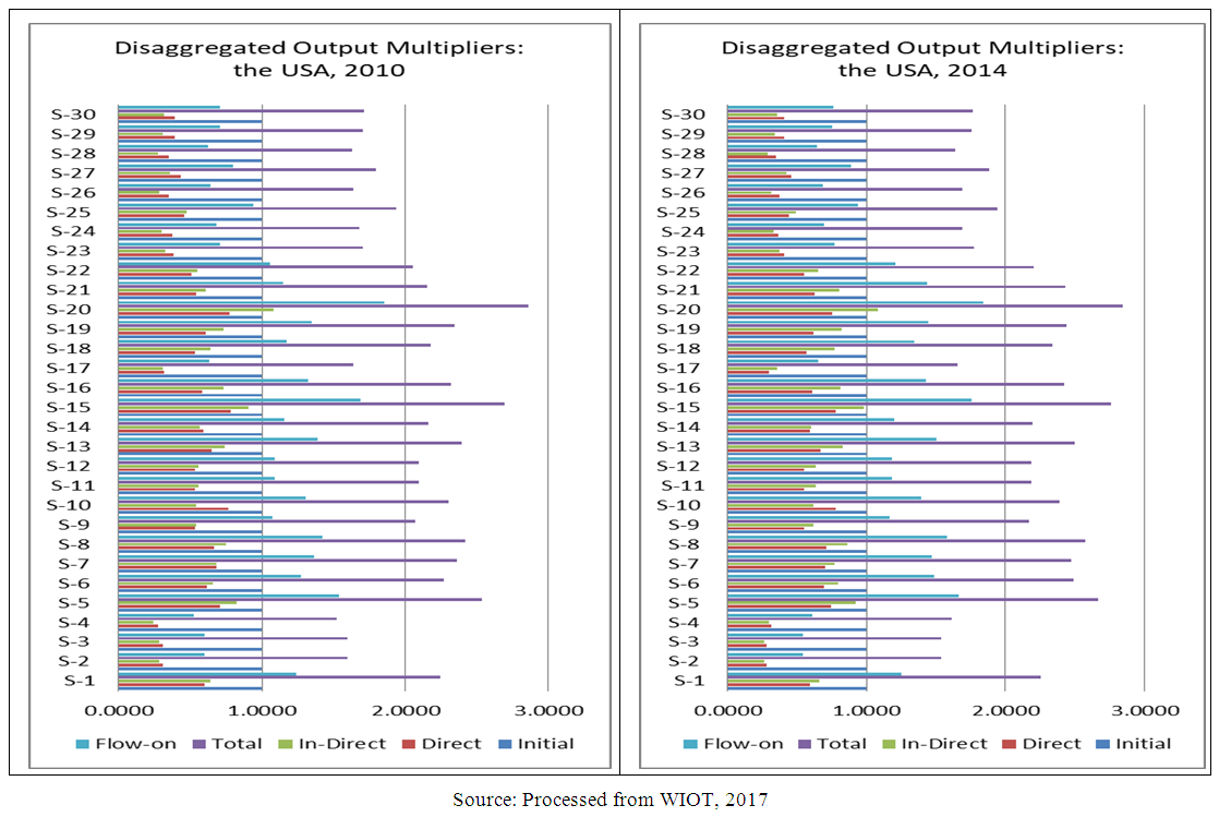
Sector-specific multipliers separate multipliers that occurred in own-sector and that occurred in other sectors. Table 1 provides sector-specific multipliers in the USA economy for the year of 2000, 2005, 2010 and 2014. In the year of 2000, average national total output multiplier that occurred in own-sector was 53.77 per cent; 46.23 per cent of multiplier occurred in other-sector. The highest percentage of multiplier occurred in own-sector was in Sector-28 (78.11%). This sector was the sector with lowest percentage of multiplier that occurred in other-sector (21.89%). The lowest percentage of multiplier occurred in own-sector was Sector-10 (42.57%); meaning that this sector had highest percentage of multiplier occurred in other-sector. In this year, there were 6 sectors with percentage of multiplier occurred in own-sector more than 60 per cent, namely: Sector-2 (61.28%), Sector-23 (61.45%), Sector-26 (65.33%), Sector-27 (62.84%), Sector-28 (78.11%), and Sector-30 (63.81%). Other sectors had percentage of multiplier occurred in own-sector less than 60 per cent. These sectors had percentage of multiplier occurred in other- sector more than 40 per cent.

Table 1. Sector-Specific Multipliers in the USA Economy: 2000, 2005, 2010 and 2014

In the year of 2005, average national total output multiplier that occurred in own-sector was 54.80 per cent; 45.20 per cent of multiplier occurred in other-sector. The highest percentage of multiplier occurred in own-sector was in Sector-28 (78.74%). This sector was the sector with lowest percentage of multiplier that occurred in other-sector (21.26%). The lowest percentage of multiplier occurred in own-sector was Sector-13 (44.33%); meaning that this sector had highest percentage of multiplier occurred in other-sector. In this year, there were 6 sectors with percentage of multiplier occurred in own-sector more than 60 per cent, namely: Sector-4 (66.64%), Sector-17 (64.04%), Sector-26 (64.55%), Sector-27 (65.29%), Sector-28 (78.74%), and Sector-30 (61.02%). Other sectors had percentage of multiplier occurred in own-sector less than 60 per cent. These sectors had percentage of multiplier occurred in other- sector more than 40 per cent.

In the year of 2010, average national total output multiplier that occurred in own-sector was 56.47 per cent; 43.53 per cent of multiplier occurred in other-sector. The highest percentage of multiplier occurred in own-sector was in Sector-28 (78.50%). This sector was the sector with lowest percentage of multiplier that occurred in other-sector (21.50%). The lowest percentage of multiplier occurred in own-sector was Sector-13 (45.30%); meaning that this sector had highest percentage of multiplier occurred in other-sector. In this year, there were 9 sectors with percentage of multiplier occurred in own-sector more than 60 per cent, namely: Sector-2 (66.70%), Sector-3 (64.62%), Sector-4 (73.27%), Sector-17 (69.30%), Sector-26 (64.32%), Sector-27 (65.94%), Sector-28 (78.50%), and Sector-30 (60.20%). Other sectors had percentage of multiplier occurred in own-sector less than 60 per cent. These sectors had percentage of multiplier occurred in other- sector more than 40 per cent.

In the year of 2014, average national total output multiplier that occurred in own-sector was 54.96 per cent; 45.04 per cent of multiplier occurred in other-sector. The highest percentage of multiplier occurred in own-sector was in Sector-28 (78.27%). This sector was the sector with lowest percentage of multiplier that occurred in other-sector (21.73%). The lowest percentage of multiplier occurred in own-sector was Sector-13 (43.56%); meaning that this sector had highest percentage of multiplier occurred in other-sector. In this year, there were 8 sectors with percentage of multiplier occurred in own-sector more than 60 per cent, namely: Sector-2 (68.85%), Sector-3 (67.30%), Sector-4 (69.71%), Sector-17 (68.81%), Sector-24 (61.35%), Sector-26 (62.88%), Sector-27 (63.69%), and Sector-28 (78.27%). Other sectors had percentage of multiplier occurred in own-sector less than 60 per cent. These sectors had percentage of multiplier occurred in other- sector more than 40 per cent.

On average, percentage of multipliers occurred in own- sector was 53.77 per cent in the year of 2000, 54.80 per cent in the year of 2005, 56.47 per cent in the year of 2010 and 54.96 per cent in the year of 2014. Sectorally, in the year of 2000, there were 20 sectors in which more 50 per cent of multipliers occurred in own-sector. The number increased to 22 in the year of 2005 and 2010 but decreased to the year of 2014. It means that on average sectoral economic activities in the USA economy more evenly distributed as almost a half on multipliers occurred in other-sector.

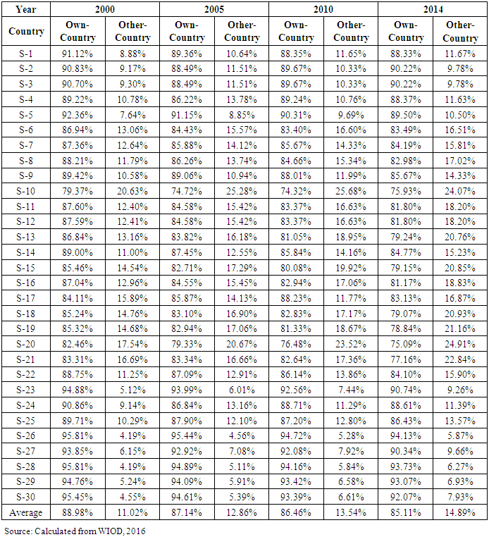
3.3. Spatial-Specific Multipliers

Spatial-specific multipliers separate multipliers that occurred in own-country and that occurred in other-countries. Table 2 provides spatial-specific multipliers in the USA economy for the year of 2000, 2005, 2010 and 2014.

Table 2. Spatial-Specific Multipliers in the USA Economy: 2000, 2005, 2010 and 2014

In the year of 2000, average national total output multiplier that occurred in own-country was 88.98 per cent; 11.02 per cent of multiplier occurred in other-countries. The highest percentage of multiplier occurred in own-sector were in Sector-26 (95.81%) and Sector-28 (95.81%). This sector was the sector with lowest percentage of multiplier that occurred in other-sector (4.19%). The lowest percentage of multiplier occurred in own-sector was Sector-10 (79.37%); meaning that this sector had highest percentage of multiplier occurred in other-sector. In this year, almost all sectors had percentage of multiplier occurred in own-country more than 80 per cent, except Sector-10 (79.37%). Almost all sectors had percentage of multiplier occurred in other-country less than 20 per cent, except Sector-10 (20.63%).

In the year of 2005, average national total output multiplier that occurred in own-country was 87.14 per cent; 12.86 per cent of multiplier occurred in other-sector. The highest percentage of multiplier occurred in own-sector was in Sector-26 (95.44%). This sector was the sector with lowest percentage of multiplier that occurred in other-sector (4.56%). The lowest percentage of multiplier occurred in own-sector was Sector-10 (74.72%); meaning that this sector had highest percentage of multiplier occurred in other-sector. In this year, almost all sectors had percentage of multiplier occurred in own-country more than 80 per cent, except Sector-10 (74.72%) and Sector-20 (79.33%). Almost all sectors had percentage of multiplier occurred in other-country less than 20 per cent, except Sector-10 (20.67%) and Sector-20 (20.67%).

In the year of 2010, average national total output multiplier that occurred in own-country was 86.46 per cent; 13.54 per cent of multiplier occurred in other-countries. The highest percentage of multiplier occurred in own-country was in Sector-26 (94.72%). This sector was the sector with lowest percentage of multiplier that occurred in other-countries (5.28%). The lowest percentage of multiplier occurred in own-sector was Sector-13 (74.32%); meaning that this sector had highest percentage of multiplier occurred in other-countries. In this year, almost all sectors had percentage of multiplier occurred in own-country more than 80 per cent, except Sector-10 (74.32%) and Sector-20 (76.48%). Almost all sectors had percentage of multiplier occurred in other-country less than 20 per cent, except Sector-10 (25.68%) and Sector-20 (23.52%).

In the year of 2014, average national total output multiplier that occurred in own-sector was85.11 per cent; 14.89 per cent of multiplier occurred in other-sector. The highest percentage of multiplier occurred in own-sector was in Sector-26 (94.13%). This sector was the sector with lowest percentage of multiplier that occurred in other-sector (5.87%). The lowest percentage of multiplier occurred in own-sector was Sector-20 (75.09%); meaning that this sector had highest percentage of multiplier occurred in other-sector. In this year, almost all sectors had percentage of multiplier occurred in own-country more than 80 per cent, except Sector-10 (75.93%), Sector-13 (79.24%), Sector-15 (79.15%), Sector-18 (79.07%), Sector-19 (78.84%), Sector-20 (75.09%) and Sector-21 (77.16%). Almost all sectors had percentage of multiplier occurred in other-country less than 20 per cent, except Sector-10 (24.07%), Sector- 13 (20.76%), Sector-15 (20.85%), Sector-18 (20.93%), Sector-19 (21.16%), Sector-20 (24.91%), and Sector-21 (22.84%).

On average, percentage of multipliers occurred in own- country was 89.98 per cent in the year of 2000, 87.14 per cent in the year of 2005, 86.46 per cent in the year of 2010 and 85.11 per cent in the year of 2014. Spatially, almost all sectors in which more than 80 per cent of multipliers occurred in own-country. It means that on average, spatial economic activities in the USA economy less distributed as more than 80 per cent of multipliers occurred in own-sector; multipliers occurred in other-sector was only less than 20 per cent.

3.4. Discussions

This section discusses important findings in this research. Firstly, total output multipliers disaggregated into initial, direct, indirect and total effects. Flow-on effect is the different between total effect and initial effect; or flow-on effect is the summation of direct effect and indirect effect. In all sectors with total output multipliers more than 2, flow-on effect was higher than initial effect; direct and indirect effects were higher than initial effect. Less initial effort will be needed to produce total output. There were 19 sectors in the year of 2000, 18 sectors in the year of 2005, 2010 and 2014, with total multiplier more than 2. Otherwise, in all sectors with total output less than 2, flow-on effect was lower than initial effect. More initial effort will be needed to produce total output. If the objective of economic development was to increase output with less effort, sectors with total output multipliers more than 2 should be prioritized in development activities.

Secondly, there was negative correlation between total output multiplier and percentage of that multiplier occurred in own-sector; the higher total output multipliers the smaller percentage of multiplier that occurred in own-sector. Regression analysis revealed that coefficients of correlation between total output multiplier and percentage of multiplier occurred in own-sector were negative and very strong with r = - 0.80 in the year of 2000; strong with r = - 0.74 in the year of 2005, very strong with r =- 0.80, in the year of 2010 and very strong with r =- 0.83 in the year of 2014. Coefficients of regression were statistically significant as calculated t-statistic (7.099 in the year of 2000; 5.789 in the year of 2005; 7.164 in the year of 2010; 7.749 in the year of 2014) were higher than critical value of t-distribution with n-1 = 29 (t-table= 1.699 at or 2.045 at ). Otherwise, there was positive correlation between total output multiplier with percentage of multipliers that occurred in other-sector; the higher total output multiplier the smaller percentage of multiplier that occurred in other-sector. Other important finding was all initial effects occurred in own-sectors. Percentage of multipliers occurred in own-sector was higher than percentage of initial effect. In all sectors, parts of direct effect of multipliers occurred in own-sector, but indirect effect occurred in other-sector. Regression analysis showed that correlation between percentage of multiplier occurred in own-sector and the percentage of initial effect of multiplier was positive and very strong in the year of 2000 (r = 0.83), was strong in the year of 2005 (r = 0.78), was very strong in the year 2010 (r = 0.85) and was very strong in the year of 2014 (r = 0.87). Regression coefficient was statistically significant as calculated t-statistic (7.81 in the year of 2000, 6.51 in the year of 2005, 8.60 in the year of 2010, and 9.21 in the year of 2014) was higher than critical-value of t-distribution with n-1 = 29 (t-table = 1.699 at or 2.045 at ).

Thirdly, there was negative correlation between total output multiplier and percentage of multiplier occurred in own-country; the higher total output multipliers the smaller percentage of multiplier that occurred in own-country. Regression analysis revealed that coefficients of correlation between total output multiplier and percentage of multiplier occurred in own-country were negative and strong with r = -0.78 in the year of 2000, r = -0.70 in the year of 2005, r = -0.76 in the year of 2010 and r = -0.75 in the year of 2014. Coefficients of regression were statistically significant as calculated t-statistic (6.578 in the year of 2000; 5.169 in the year of 2005; 6.222 in the year of 2010; 6.067 in the year of 2014) were higher than critical value of t-distribution with n-1= 29 (t-table = 1.699 at  or 2.045 at ). Otherwise, there was positive correlation between total output multiplier with percentage of multipliers that occurred in other-countries; the higher total output multiplier the smaller percentage of multiplier that occurred in other-countries. Another important finding was all initial effects occurred in own-country. Percentage of multipliers occurred in own-country was higher than percentage of initial effect. All direct effects of multipliers were occurred in own-country, except Sector-10 in the year of 2005 and 2010. However, part of indirect effect occurred in other-countries. Regression analysis showed that correlation between percentage of multiplier occurred in own-country and the percentage of initial effect of multiplier was positive and very strong in the year of 2000 (r = 0.80), was strong in the year of 2005 (r = 0.73), was strong in the year of 2000 (r = 0.76) and was very strong in the year of 2014 (r= 0.87). Regression coefficient was statistically significant as calculated t-statistic (7.004 in the year of 2000, 5.727 in the year of 2005, 6.116 in the year of 2010, 9.211 in the year of 2014) was higher than critical-value of t-distribution with n-1=29 (t-table= 1.699 at  or 2.045 at ).

4. Conclusions

From discussion above, some conclusions could be drawn. Firstly, all sectors with total output multipliers more than 2, flow-on effect was more than initial effect. All sectors with total output multiplier less than 2, flow-on effect was less than initial effect. In the USA economy, there were 19 sectors in the year of 2000, 18 sectors in 2005, 2010 and 2014, with total output multipliers more than 2. In order to increase output, priority should be given to those sectors with total output multipliers more than 2 as less initial effort will be needed to produce output. Secondly, total output multipliers had negative correlation with percentage of multipliers that occurred in own-sector, but total output multipliers had positive correlation with percentage of multipliers that occurred in other-sector. The higher total output multipliers, the smaller percentage of multipliers occurred in own-sector; the higher total output multipliers, the higher percentage of multipliers occurred in other-sector. All initial effects occurred in own-sector. Parts of direct effects occurred in own-sector, but all indirect effect occurred in other-sector. Thirdly, total output multipliers had negative correlation with percentage of multipliers that occurred in own-country, but total output multiplier had positive correlation with percentage of multipliers that occurred in other-countries. The higher total output multipliers, the smaller percentage of multipliers occurred in own-country; the higher total output multipliers, the higher percentage of multipliers occurred in other-countries. All initial and direct effects occurred in own-country. Parts of indirect effects occurred in own-counties.

There are two basic limitations on this paper. Firstly, there were inherent assumptions in input-output model such as linearity and divisibility. Secondly, manual calculations could make mistakes easily. Developing more dynamic and realistic model such as computable general equilibrium model would provide more realistic calculation of multiplier. Developing computer software for calculation sector-specific and spatial-specific multipliers also suggested as it would make such calculation much easier.

Appendices

Appendix 1. Sector Classifications

Appendix 2. Country Abbreviations