1. Introduction

Growth is one of the main objectives in policy and economic planning and also, Banking and financial sector development is essential for economic growth. According to studies, financial development is not desirable in Iran. One of the limiting factors of financial development is reduction in the bank interest rate under conditions of inflation. Financial liberalization with financial development allows domestic financial markets to compete the international financial ones.

Besides, Money demand is an important function when analyzing effects of macroeconomic policies. Furthermore, the money demand stability is a prerequisite to predict effects of money on the economy so that the central bank could take an active monetary policy to control money supply. Money demand is an important function in transmission of monetary policies to real sectors of economy; as a result, it should be stable enough. A number theoretical and empirical studies has been performed on estimation of money demand function, most of which are conducted in U.S and European countries. Recently, few studies have been conducted in developing countries. Most of these studies have employed Cointegration Technique (Engel and Granger, 1987) and Multivariate Cointegration Test (Johansen and Josilius, 1990). Most developing countries have taken some positive steps during the 1990s and in recent years towards economic stabilization policies and financial liberalization. Nowadays, the knowledge of globalization is spreading more rapidly throughout the world due to the development in the field of communication and technology which will make the world economies more interdependent. This is generalizable to other regions such as the Middle East, a region that Iran is a part of it. As a result, it is necessary global and regional financial trends to be taken into account when reforming the country’s financial structures and to adopt specific strategies and policies in this regard (Karimi, 2008). This study aims to examine possible effects of financial liberalization on the stability of money demand in Iran. The present study is distinguished from the others in that: 1) the stability of money demand has been evaluated in four models in spite of structural break and 2) Short run and long run relationship between money demand variables has been estimated using data from 1973 to 2009. This paper contains five sections. The first part, introduction, deals with the importance of money demand. The second section presents studies done in Iran and abroad. The third section deals with theoretical framework of the study, the indicators used, and the way econometric model is computed. The fourth section analyzes results of estimation of econometric model. Finally, the last section provides conclusions and suggestions for future research.

2. Review of Literature

Money demand stability has received much attention by researchers, showing the importance of this issue in an economy. Accordingly, the present chapter provides a review of studies conducted in Iran and abroad to come up with a better understanding of the problem in question. Pradhan and Subramanian (2003) studied the stability of money demand in developing economies under the influence financial liberalization in India using three experiments. The data used in the study were related to 1970-2000 time period collected monthly. The results suggested that the stability of real long run money demand is not influenced by financial liberalization. Onafowora and Owoye (2003) conducted a study under “Structural adjustment and the stability of the Nigerian money demand function” using the definition of extensive money (M2) in Nigeria and Johansson Josilious’ Maximum Likelihood Method and Cintegration Test in 1986-2001 time period. They found that the money demand function was stable in the period under study. Rao and Saten (2007) performed a study titled “Cointegration, structural breaks, and the demand for money in Bangladesh” using limited money definition (M1) in Bangladesh using cointegration approach and Gregory-Hanson Test to examine the stability of money demand over 1973-2003 using annual data. The results of the study during the 1988-2003 time period the money demand was stable. However, the money demand for limited money underwent a relative decline in the 1980s, as expected by the authors of the study. Akinlo (2006) examined the stability of money demand in Nigeria using the autoregressive distributed approach along with CUSUMSQ and CUSUM tests for the time period of 1970 to 2002. The result of the study indicated that the money demand was stable in the period under consideration. Tang (2007) investigated the stability of money demand function in Japan based on rolling cointegration approach using autoregressive distributed approach and CUSUMSQ and CUSUM tests for the time period of 1960 to 2007. The results of the study indicated that M2 was correlated with income and interest rate. Furthermore, the money demand was stable in the period under study. However, the weaknesses of CUSUMSQ and CUSUM tests in demonstrating dependent variables made the researcher to perform a correlation test that indicated that contrary to other studies, the money demand in Japan was not stable in this period.

Zubaidi Baharumshah, Hamizah Mohd, & Mansur Masih, (2009) examined the stability of money demand in China using the data collected by the ARDL model and the definition of extensive money (M2) for the time period of 1990-2007. The results of the study indicated that there is a stable and long run relationship between M2, the real income, inflation rate, foreign interest rate, and stock prices. They found that stock prices considerabley affected on the extensive and limited money demand. Finally, Darrat and Al-Sowaidi (2009) conducted a study under “Financial progress and the stability of long run money demand: Implications for the conduct of monetary policy in emerging economies” to investigate changes made in the money demand stability due to financial changes in three emerging economies in the Persain Gulf countries (e.g. Bahrain, the UAE, and Qatar) for the time period of 1994 to 2008. They observed that rapid financial changes in these three emerging economies do not lead to changes in the stability of money demand. Besides, the adoption of M1 for the UAE, M2 for Qatar, and M1 and M2 for Bahrain is suitable for controlling monetary policies. Eslamluian and Heidary (2003) in a study titled “Lucas criticism and analysis of money demand stability in Iran” have examined the stability of money demand function coefficient in Iran during 1961-1976. To do so, they employed exogeneity and super exogeneity tests. They also employed auto regressive distributed lag (ARDL) model to estimate the short run and long run relationships between variables. The results of the study indicated that the money demand over the period consideration is unstable compared to the exchange rate in the same period. Komeyjani and Boustani (2004) in his M.S thesis under “Money demand stability in Iran” has examined the stability of money demand behaviors over 1960-2002 time period and has employed Johansson and Josilius (1990) cointergation test. He found that despite the long run stability in the money market, the movement towards stability takes place slowly in this market. The results of CUSMSQ and CUSUM tests indicate that money demand in Iran was stable in the period under study.

Sadeghzadeh Yazdi, Jaafari Samimi, and Elmi (2006) in an empirical study on the stability of money demand in Iran investigated money demand function in Iran using Johansson Josilious Maximum Liklihood Method during 1959-2002. The results indicated that money demand in Iran was stable in the period under study. Davoudi and Zarepour (2006) examined the effects of money definition on the money demand stability with a focus on Divizhya index in the 1988-2004 time period using the seasonal data. They suggested that the use of simple sum technique to define money is inconsistent with microeconomic theories since it is implied that consumers regard the money demand component as complementary to each other. The results of the study showed that the money demand was stable in all three models. However, the adjustment pace was much greater in Divizhya models than was in simple sum models. In addition, since empirical evidence suggests that the money market will get stable very quickly and monetory shocks are absorbed very rapidly within the economy, it can be said that Divizhya models have estimated correctly the money demand function. Shahrestani and Sharifi Renani (2008) conducted an empirical study on “The estimation of money demand function and its stability in Iran” to determine the relationship between money and other macroeconomic variables (e.g. real income, inflation, and exchange rate) for Iranian economy over the time period of 1985-2005 using econometric auto regressive distributed lag technique (Pesaran and Shin, 1995). The results of the study indicated the stability of the money demand function (M1) but it was not the case for the money demand function (M2).

Azvaji and Farhadikia (2007)” Evaluation of effects of financial liberalization policies and changes in interest rates on financial development in Iran (VECM model)”.

The objective of this study is to evaluate the effect of the financial liberalization policies and changes in real interest rates (including Deposits and loans) on financial sector development for Iranian economy during the 1969-2003 time period using VECM model.

In this study, the model is based on Arestis research (2002). Since in some developing countries, money market structure is similar to Iran economy, this model has been considered for Iran. The final model for empirical estimation in Iran economy defined as:

Where:

LFDt: logarithm of financial development(logarithm of the ratio of nominal claims on private sector to nominal GDP).

LNIPOPt: logarithm of economic development (ratio of real GDP to total population in country).

RIRRt: real interest rate (with adjusting for inflation) on informal sector in Iran.

RIRDt: Deposit Interest Rate (with adjusting for inflation).

RLRt: legal minimum fraction of deposits which the banks are mandate to keep as cash with themselves. RLRt is fixed by the Central Bank.

In this research, the results demonstrate there is a significant negative relationship between the legal reserves (controlled by central bank) and financial development. Also there is a significant relationship between changes in real interest rate (Loans and deposits) and financial sector development. In addition, increase in real interet in informal market lead to decreases in demand and turning informal market to formal one (banking system) and also lead to financial market development in Iran economy.

Komeijani and Pourrostami (2008) “effect of financial repression on economic growth (comparing less and least developed countries).

In this paper, panel data have been analyzed to investigate various forms of financial repression regarding to interest rate as well as theirs effect on economic growth of different countries (33 less developed country, 38 least developed country and 21 developed country) during 1985-2005. The equation is estimated using ordinary least square method (OLS):

GDP⁰ = C₁ + C₂GDP0 + C₃Set + C₄Prm + C₅Gov.EXP + C₆Distort + C₇Gov.Stability + C₈FIR

Where:

GDP0: average income growth rate (economic growth)

GDP0: initial value of GDP

Set: registration rate at high schools

Prm: registration rate at primary schools (human capital)

Gov.exp: ratio of true cost of government to real GDP.

Distort: deviation of price of capital goods from the average over the period.

Gov.stability: Government Stability Index

FIR: financial repression index.

The results of this study show that various form of economic interventionism such as: determining of interest rate ceiling, high reserve requirement, restricting or regulating of current and capital account transactions, interventing on Distribution of bank Credits, restrict the financial markets and also cause a negative bank interest rate which called financial repression against liberalization. Furthermore, the estimations shows negative significant effect of negative interests rate on economic growth of countries. Finally, the assessments demonstrate that increase in negativity of interest rate may have a negative impact on economic growth.

James B. Ang and Warwick J. McKibbin (2007) “Financial Liberalization, Financial Sector Development and Growth: Evidence from Malaysia”.

The objective of this paper is to examine whether financial development leads to economic growth or vice versa in the small open economy of Malaysia. Also, the results support the view that output growth causes financial depth in the long-run.

Based on series data from 1960 to 2001 and VECM method, the financial depth relationship can be described as follows:

Where FD_t refers to financial development index and ED_t is the level of economic development (measured by logarithmic per capita real GDP). RI_t refers to the real interest rate and FR_t is an index which measures the extent of financial repression. The equations can be expressed as fallows:

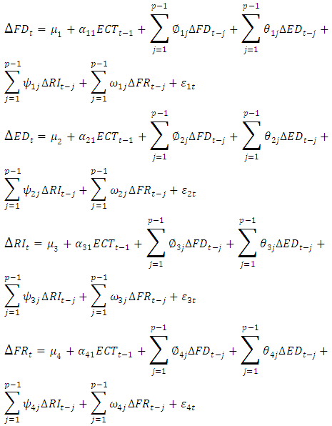It should be mentioned that, we use logarithm of liquid liabilities (or M3) to nominal GDP, logarithm of commercial bank assets to commercial bank assets plus central assets plus central bank assets, and logarithm of domestic credit to private sectors divided by nominal GDP as the proxies for financial development and also, interest rate and credits controls, reserve retirement to liquidity as proxies for financial depth.

The results show that financial liberalization may have a desirable impact on financial development. In fact, negative real interest rate has a negative effect on financial development. Finally, there is a unilateral casual relationship between financial development economic growth means that economic growth can lead to financial development.

Yung Y. Yang, Myung Hoon Yi (2008) “Investigation on causal relationship between financial development and economic growth for Korea”.

They examined the casual relationship between development and economic growth using annual data for Korea during 1971-2002, during which Korea has experienced both phenomenal economic growth and a variety of financial liberalization. In this study, capital stock to nominal GDP has been used as financial development index. The resulting equations are as follows:

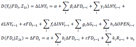Where INV is the ratio of gorss fixed investment to GDP, G the ratio of government consumption to GDP, and OPEN is the ratio of export plus import to GDP. R, Represents the real interest rate, which is control variable and Z_t is the conditioning variable.

The results recommend that policy priority should be given to financial reform, because only decisive and accelerated pace of financial restructuring can ensure a sustainable growth in the medium or long term. With the finding that the financial development control causes the economic growth, but the reverse is not true, we can conclude that there is a unidirectional causality from the financial development to the economic growth.

Summaries and conclusion of studies reviewed: Many studies have been done on money demand stability in Iran and other countries. The results show that within the periods under study, money demand function has had certain stability. But the results of studies done in Japan, on the contrary, showed the money demand was instable in Japan in the period under consideration.

Domestic results about effect of financial liberalization on economic growth express that economic growth can lead to financial development and most of studies are based on developing countries, especially countries in East Asia which emphasize on domestic studies more than financial liberalization.

All studies confirm that financial liberalization policies result financial development.

Theoretical framework of the study

Theoretical framework of money demand function: Money demand theories of have undergone some changes over time. For instance, one of the oldest theories is the famous quantitative theory of money. Of the famous pioneers of this theory among classics, we can refer to Iroing Fisher, Alfred Marshal, and Pigou. Money is regarded as a unit of counting in the classical school. Economists at Cambridge University have presented cash balance approach based on which monetary demand is regarded as a general demand for maintaining money. They also determined the relationship between real income and demand for real money. However, keynes, who was educated in the Cambridge School and followed it, has mentioned more accurately three motives for money demand:

Ÿ transaction motive; 2) precautionary motive; and 3) speculative motive (Sadeghzadeh Yazdi, jaafari Samimi & Elmi, 2006).

In addition, Bamul-Tubin Transaction Demand is another theory that assumes monetary transaction demand is also a function of the rate of interest. While in the Cambridge and Keynes theories, transaction demand is regarded as the function of income. (Sadeghzadeh Yazdi, Jaafari Samimi & Elmi, 2006). Friedman’s money demand is another theory based on which money for consumer has a kind of psychological utility because of ease of doing the transactions. Money also acts as a kind of production input for producers. Therefore, the usefulness of money should be compared with the productivity of the assets that substitute for money. (Sadeghzadeh Yazdi, Jaafari Samimi & Elmi, 2006). Consequently, money demand is a positive function of wealth or permanent income and a negative function of the expected yield of other assets.

Instability in money demand function: Since the early 1970s, the money demand function in United States predicted the money demand more than what was in reality. The rate of errors increased significantly from 1974 to 1976. (Komeyjani & Boustani, 2004). According to Goldfeld’s (1976) theory, the definition of M1 wasn’t stable and we can’t evaluate money demand function during these years. Goldfeld has regarded this change as missing money and believes that this has resulted in lack of any prediction about M1 demand. Afterwards, a better understanding gained about how monetary policies would affect economical activities through adoption of an instrumental view to the money demand function. Any attempt to find a stable function of money demand is made in two ways. First of all, economists regarded the incorrect definition of money as the cause of instability in money demand. On the other hand to find new variables, researchers tried to gain a stable function of money demand by embedding such variables into the money demand function. Hamburger (1977) believed that by adding dividends rates into its average price, the money demand function will be stable. Other economists (e.g. Khan and Heller, 1979) have also performed some studies to explore the issue. However, since the new and additional variables didn’t correctly reflect the cost of opportunity of saving money and as there was no strong theoretical explanation for inclusion of these variables in the model, this theory received some criticisms. (Komeyjani & Boustani, 2004). In the early 1980s, studies and literature on the money demand function faced another challenge. In this period, the economists were faced with a decreased velocity of money not predicted by the money demand function. Statistical data collected in this period suggested that M2 velocity of money was much more stable than M1 velocity of money. As a result, researchers found that by presenting a wider definition of money, money demand function will benefit from more stability in the 1980s. Considerable changes occurred during the 1970s. Komeyjani & Boustani, (2004) On one hand, financial innovations and, on the other, rises in the yield of bonds were highly effective in forming a wide range of financial assets.

During the period under study, the costs of data processing and telecommunications decreased. Johanson and Paulus (1976) believed that in instability in money demand function for the UAE had occured because of financial innovations. (Komeyjani and Boustani, 2004). Boughton (1981) classifies broadly instability as follows:

1) Institutional changes which result in a change in the way the public will use assets.

2) International developments which refer to sudden changes in the exchange rate.

3) Changes in monetary policies: restricting the growth of one part of financial sector by monetary authorities without exerting similar restrictions over other sectors. (Komeyjani & Boustani, 2004)

Arango and Nadiri (1981) believe that money demand function instability is because of changes made in the foreign currency system as confirmed by Gorden (1984) who has pointed out that a part of instability in short-run money demand function may be the result of changes in the Philip’s Curve due to impulses of money supply during 1973-1975. Some researchers such as Griton and Roper (1981) suggest that money substitution is the cause such instability. (Komeyjani & Boustani, 2004). Since 1990’s to the recent years, globalization knowledge is transferred more quickly because of technological developments which makes the world economics more interdependent, a pint which is generalizable to other regions like the Middle East where our country is located. Accordingly, it is necessary to consider the regional and universal financial trends in reforming the financial structures of our country and adopt distinct strategies and policies in this regard.

Variables selection: The main reason behind theoretical and experimental studies is to gain a stable demand function as a prerequisite for taking effective monetary policies. Money demand stability will facilitate evaluation of effectiveness of monetary policies on different economies. (Shahrestani and Sharifi Renani, 2008). Accordingly, money demand functions have been tested via different variables. Most studies have come to an agreement about the importance of definition of money and variables of scale and opportunity costs of saving money. Some of these have investigated foreign opportunity costs of saving money including exchange rate and foreign rate of interest. (Shahrestani and Sharifi Renani, 2008) Choosing effective variables is of high importance in money demand functions. Theoretical frameworks discussed in the present study show concepts such as definition of money and variables of scale and opportunity costs of saving money. Money has been defined differently in experimental studies. The present study has employed real volume of money, liquidity, real short run interest rate, real long run interest rate, wholesale price of industrial productions, real exchange rate, real rate of facilities, growth rate of Gross domestic product, and indicators of efficiency of financial developments.

Money demand: Money demand model is written as follows:

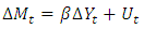(1)

Where is the difference, M is real money, stands for the effective coefficient Y shows scale variable and opportunity cost, is the disturbance term, M represents volume of money, and M1 and M2 are liquidity. Besides, Y is the wholesale price of industrial productions and opportunity cost (including inflation rate, real short-term interest rate, real long-term interest rate, real exchange rate, and real rate of facilities).

In order to use interest rate in the present study, (short run and annual) deposit rates and rate of return on facilities (loans) have been employed. It should be noted that the financial indicator used is the ratio of credits paid to the private sector to GDP. Besides, to make the inflation variable significant, a dummy variable d71 was included in the equation for 1992 to 1995 time period. Five models are tested in the study as follows:

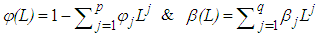
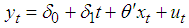
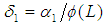
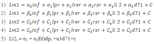So that:

Lm1: logarithm of real money, Lm2: logarithm of liquidity, inf: inflation rate,

Lpr: logarithm of the wholesale price of industrial productions, Lrer: Logarithm of real exchange rate, Rsr: real short run interest rate, Rlr: real long run interest rate.

Fa: real rate of facilities, Li2: logarithm of financial indicators،EGdp: growth rate of gross domestic product.

Tests

Auto-Regressive Distributed Lags Model (ARDL): Pesarn and Shin (1999) have suggested the use of the traditional Auto-Regressive distributed lags (ARDL) in order to analyze long-run relationships between nonstationary variables. ARDL Model with a number of P lags for dependent variable (y_t) and a number of q lags for explanatory variables (x_t) is written as follows:

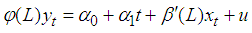(2)

where L is lag operator and t is the time trend,

(3)

After application of equal conditions of lags for each variable, long term relationship between variables is obtained as follows which can be used to estimate long term coefficients in the model:

(4)

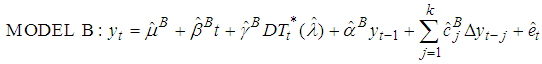
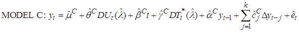
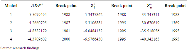
Where and (Pesaran & Shin, 1999)

When estimating the coefficients using ARDL, in the first stage, optimal p and q lags are selected by using Akaeik Index or Schwarz Bayesian Index. In the next stage, long term coefficients of the variables and their critical points are estimated via ARDL Model as used in the first stage.

Zivot-Andrews Unit Root Test: Zivot and Andrews (1992), emphasizing the role of structural breaks to examine stationary of the variables, believe that Perron Method is not a complete approach as it does not perform pre-tests and predetermined selection of break points. Therefore, they introduced a unit root test in which, unlike Perron Test, the time of structural break is not predetermined. Experimental studies done by Zivot and Andrews showed that the method used by them to reject the null hypothesis indicating the presence of unit root is stricter than that of Perron. Since through this method, they found out that the four variables introduced with a stationary structure break by Perron was, in fact, nonstationary. (Zivot-Andrews, 1991) To develop unit root test, Perron modified the generalized Dickey-Fuller Unit Root Test (ADF) and introduced three behavioral equations, each containing possibly one exogenous structural break. While adopting three equations developed by Perron, Zirot-Andrews Method first determines the time for occurring one endogenous break point (T_B) for each variable.

As a result, Perron’s behavioral equations to examine stationary of variable y are presented as follows:

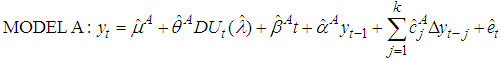(5)

(6)

(7)

Where λ stands for the ratio of the annual break to the whole time period (T_B/T), μ is intercept, and t is variable of trend. Variable DU shows the break in intercept that takes a value of 1 for years after T_B and a value of 0 for other periods. The variable related to the break in the slope of the trend function is shown as DT*, that assumes a value of t - T_B for years after T_B and a value of 0 for other years. In these equations, differential variables of the past periods to the K^th rank have entered into the models to solve the problem of auto-regression. In Zivot- Andrews Method, first A, B, and C models have been estimated separately through ordinary least squares method (OLS) for a given range of T-student statistics associated with the null hypothesis will be calculated for each . Then, the corresponding year with the least (negative) statistics will be introduced as the break year (T_B) and its computational statistics is selected as a valid statistics to test the null hypothesis. The minimum statistics can be determined with the use of the following equation in which ^ is the variable range for (Zivot- Andrews, 1991)

(8)

In this method in which the time of break is determined endogenously, Perron’s critical values are not valid. Because their absolute values are very low and the null hypothesis on the existence of unit root is simply rejected. (Zivot-Andrews, 1991) Zivot and Andrews presented a number of tables containing new critical values for every triple model. If the minimum computational value of for every model is more than the critical value, the null hypothesis indicating the existence of unit root without any exogenous structural break will be rejected in the favor of alternative hypothesis which assumes “the stationary state of a variable in the presence of a structural break in an unknown time period”. (Zivot-Andrews, 1991)

Gregory-Hansen Cointegration Test¹: Give the nonstationary nature of most of the time series variables and absence of comprehensive and efficient solutions for stationing nonstationary variables, cointegration methods were introduced to help the researchers to estimate economic models without being concerned about the existence of pseudo regressions. To enter the effect of this unknown break φ_tτ the virtual variable is used which is defined as follows:

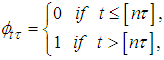(9)

The variable was not predetermined but it is equal to the ratio of the break time [nt] to the whole period under study (n) and [] as the operator of the integer. Based on what was mentioned above, three equations developed by Gregory-Hansen were introduced for a model with a dependent variable (y_1t) and m number explanatory variables (y_2t) as follows:

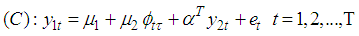(10)

(11)

(12)

C Model known also as “level shift model” shows a structural break in an unknown time period, resulting in a change as much as µ2 in the intercept vector of cointegration regression, but it doesn’t affect the regression slope vector (α). C/T model also known as “Level shift with the trend model” is formed by entering a time trend (t) in C model. C/S Model is the same of “regime shift model” that in addition to the intercept change makes a possible a change with the size of α2 in the slope vector of cointegration regression. (Gregory – Hansen, 1996) In Gregory-Hansen Method, a similar process is applied using residual terms in equations (11), (12), and (13) and in addition to ADF statistics, two Philips unit root statistics are also used to examine the null hypothesis about non-cointegration. In order to calculate required statistics, first we choose one of the triple equations of (10) to (13) and estimate its coefficients for all τs through OLS. Then we extract estimation residual terms corresponding to all the τs that are the members of (T) interval. To calculate “the bias-corrected first-order serial correlation coefficient” we substitute them in the following equation:

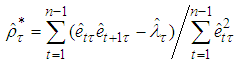(13)

Where stands for the weighted sum of auto-covariance for each τ that has added into the first-order serial correlation coefficient relation in order to adjust the statistics of Phillips Test. Using this coefficient, Phillips Test statistics are developed as follows:

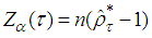(14)

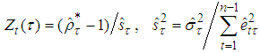(15)

Where, is the long term variance of second-stage residual terms. To calculate generalized Dickiey-Fuller statistics (ADF), we write a regression equation for each break point ( T ) follows:

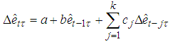(16)

ADF statistics is t statistics related to the variable which is used to test the null hypothesis b=0 and can be shown as follows:

(17)

Statistics used in Gregory-Hansen Cointegration Test are the same as and, minimum computational statistics for all members of interval T and are shown as follows: (Gregory – Hansen, 1996)

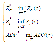(18)

Whenever, the value of above statistics is higher than the critical values, the alternative hypothesis is confirmed, indicating the existence of a cointegration relation in the presence of structure break.

Structural stability tests

Cumulative sum test (CUSUM) and cumulative sum of squares test (CUSUMQ): In order to examine the stability of model coefficients, CUSUMQ and CUSUM tests employed for a long time in the literature on econometrics are used. In these tests, the null hypothesis examines the stability of parameters at a significance level of 5%. The confidence interval in these two tests is two straight lines that show a confidence interval of 95%. If the test statistics is between these two lines, it is not possible to reject the null hypothesis showing the stability of the coefficients.

Data analysis: In this section, the results of estimation of coefficients for the money demand variables have been assessed during 1973 to 2009. The results of Zivot-Andrews Unit Root Test are shown in the following table:

Table 1. Zivot-Andrews Unit Root Test

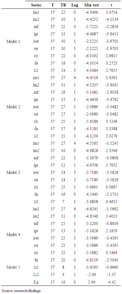
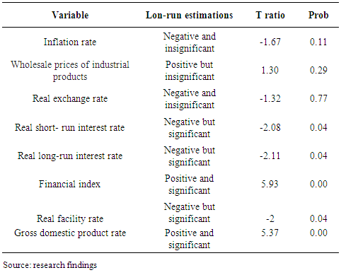
In all models, the minimum calculated value of for each model is less than the critical value. As a result, the null hypothesis is not rejected at 5% level of significance which assumes the existence of a unit root without any exogenous structural break. The results of Gregory-Hansen Cointegration Test are shown in the following table:

Table 2. Gregory-Hansen Cointegration Test

The values of the above statistics are less than the critical values so the null hypothesis is not rejected at 5% level of significance. Besides, there is no structural break in all four cointegration models.

Model estimation: The model under consideration was estimated via 4.1 Microfit Software. By entering the data collected in Iran from 1974 to 2009, 3 Lags was considered as the maximum lag. In the next stage, optimum lags are determined using criteria such as Akaeik, Hanan-Queen, and adjusted determination coefficient. Schwarz Baycsian Criterion (SBC) is normally used for samples less than 100 observations in order not to lose much degree of freedom.

Short-run estimations

Overall results for short-run estimations: Table 3 shows the overall results for short-run estimations:

Table 3. Overall results for short-run estimations

Discussion: Inflation rate, real exchange rate, real short run interest rate, real long run interest rate, and financial index have a positive and significant effect on real money demand, wholesale prices of industrial products have a negative and insignificant effect on real money demand. Furthermore, real facility rate have a positive and significant effect on real money demand. The more is rate of inflation, the less is the value of money. Besides, more money is needed for previous transactions, and as a result the demand for money will increase. An increase in the exchange rates causes an increase in money demand that is in line with “wealth effect”. According to McKinon- shaw (1973) Theory at the time of financial liberalization, an increase in saving and economic growth will increase results money demand. The improvement of financial index shows economic growth that has a positive correlation with money demand. Generally, it can be said the financial liberalization in the period under consideration affects money demand stability significantly during a short run period.

The results of Classic Assumptions Recognition Test

Table 4. Results of Classic Assumptions Recognition Test

Long run estimation of model

Table 5. Results of long run estimation

Discussion: Inflation rate and real exchange rate have a negative and insignificant influence on the money demand. Real short run interest rate, real long run interest rate, and real facility rate affect the money demand negatively and significantly. Financial index has a positive and significant effect on the money demand. Finally, wholesale price of industrial products positively and significantly affect the real demand for money. Inflation rate, real exchange rate, real short run interest rate, real long run interest rate, and real facility rate are, in effect, the cost of maintaining money which have a negative effect on the money demand in long run. An increase in the exchange rate will result in a decrease in the money demand which is in line with “substitution effect”. The higher the wholesale price of industrial products, the lower the money demand. An increase in the financial index is indicative of the conditions of economic growth which results in higher demand for money. Generally, it can be said that: financial liberalization in the period under consideration has affected the stability of money demand significantly in a long run.

Error Correction Model: Error Correction Model shows long run and short run relations between dependent and independent variables in the model. The results of error correction for model 1 are as follows:

Lm1 = -.070708*Inf +.094957*Lpr -.26798*Lrer -6.7688*Rsr -.90081*Li2-10.2200*C -.036118*D71+ ecm

The important point in error correction model is the coefficient of error correction term that shows the adjustment speed of imbalance process towards a state of balance in a long run. As shown in the above table, this coefficient is negative and significant and since the ECM coefficient is between 0 and -1 and, thus, significant, the existence of cointegration relation between the variables is confirmed. In addition, as the coefficient for error correction term is equal to ( -0/466), it can be concluded that in each period, almost 46% of the existing imbalance in the dependent variable will be adjusted and eliminated from its long run balanced values in the next period. In other words, in the case that any kind of shock or imbalance is created in money demand function it will return to a balance state. As a result, it can be said the moving towards the balance is relatively desirable.

The results of error correction for model 2 are as follows:

Lm1=.0040675*Inf -.75493*Lpr -.13410*Lrer -4.8440*Fa -.65862*Li2-7.2644*C-.56456*D71+ ecm

Since the ECM coefficient is between 0 and -1 and significant, the existence of cointegration relationship between the variables in question is confirmed. What’s more, as the coefficient of error correction term is equal to (-0.266), it can be concluded that in each period almost 26% of the created imbalance in dependent variable will be adjusted and removed from its long term balanced values in the next period. In other words, if any kind of shock or imbalance is created in money demand function it will return to a balance state. The results of error correction for model 3 are as follows:

Lm2= -.079136*Inf +.17018*Lpr +.051017*Lrer -7.7860*Rlr-1 Li2 -14.2849*C -.043494*D71+ ecm

Since the ECM coefficient is between 0 and -1 and significant, the existence of cointegration relationship between the variables in question is confirmed. What’s more, as the coefficient of error correction term is equal to (-0.437), it can be concluded that in each period almost 43% of the created imbalance in dependent variable will be adjusted and removed from its long term balanced values in the next period. In other words, if any kind of shock or imbalance is created in money demand function it will return to a balance state. The results of error correction for model 4 are as follows:

Lm2 = -.011632*Inf +.11540*Lpr +.23435*Lrer -3.4934*Fa -1.3882*Li2 -16.4045*C +.0044027*D71+ ecm

Since the ECM coefficient is between 0 and -1 and significant, the existence of cointegration relationship between the variables in question is confirmed. What’s more, as the coefficient of error correction term is equal to (-0.183), it can be concluded that in each period almost 18% of the created imbalance in dependent variable will be adjusted and removed from its long term balanced values in the next period. In other words, if any kind of shock or imbalance is created in money demand function it will return to a balance state. The results of error correction for model 5 are as follows:

Li2_t = 0.029EGdp_t +0.091d71+c

Since the ECM coefficient is between 0 and -1 and significant, the existence of cointegration relationship between the variables in question is confirmed. What’s more, as the coefficient of error correction term is equal to (-0.336), it can be concluded that in each period almost 34% of the created imbalance in dependent variable will be adjusted and removed from its long term balanced values in the next period.

Cumulative Sum Test (CUSUM) and Cumulative Sum of Square Test (CUSUMQ): The following diagrams show the results of CUSUM and CUSUMQ tests. The statistics are plotted for specific time periods and as shown in the diagrams, the statistics obtained through the tests are placed inside straight lines, indicating the stability of the coefficients at a significant level of 5%. In other words, it is not possible to reject the null hypothesis at a confidence level of 95%, indicating the stability of coefficients.

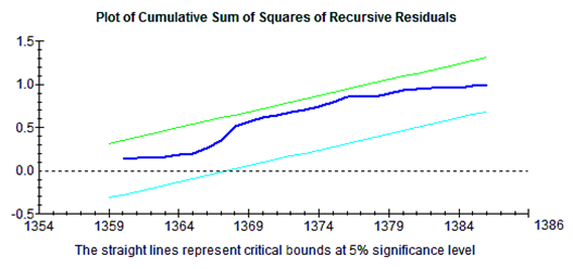
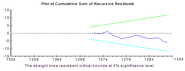Figure 1. Model 1

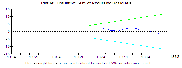Figure 2. Model 2

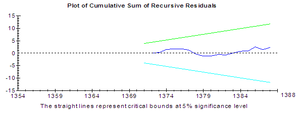Figure 3. Model 3

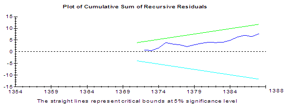Figure 4. Model 4

Figure 5. Model 5

3. Conclusions

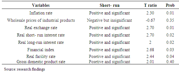
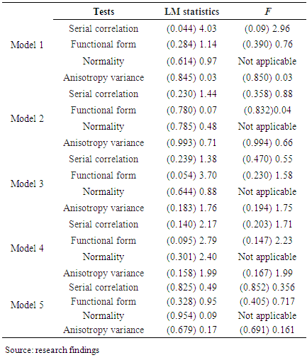
The results of the present study are summarized as follows:

1) Financial liberalization in the period under study has a significant effect on money demand function.

2) Zivot-Andrews Unit Root Test confirms the existence of unit root without any exogenous structural breaks.

3) Economic growth has significant positive impact on economic development

4) Gregory- Hansen Conitegration Test shows that given the structural and regime changes, there is not long term balance relationship at a confidence level of 95%.

4. Recommendations

Money demand stability is a prerequisite so that money demand could have a predictable effect on economy and the central bank could control money demand in order to implement active monetary policies. On the other hand, if the money demand function is unstable the changes will be unpredictable and monetary officials will not be able to predict the effects of money changes on other variables. In iran, demand side of the financial market is true on the other hand increase in demand due to economic growth leads to financial market development. Regarding to the results. A higher economic growth has an important role in the financial sector, especially bank sector in Iran. Therefore, using the adequate policies in order to achieve a higher economic growth are essential. hence, it is recomended that, in order to financial development in Iran, growth which is the main factor in financial sector should be more considered, because government impose the interest rate to the bank in Iran, it is recomended that government control decrease and interest and inflation rate change simultaneously (according to market).

Note

1. The content of the article, Gregory - Hansen has been getting. For a more detailed explanation see: Samadi et al. (2005). pp. 77-72.