-
Paper Information
- Previous Paper
- Paper Submission
-
Journal Information
- About This Journal
- Editorial Board
- Current Issue
- Archive
- Author Guidelines
- Contact Us
American Journal of Economics
p-ISSN: 2166-4951 e-ISSN: 2166-496X
2017; 7(1): 46-62
doi:10.5923/j.economics.20170701.06

Vector Autoregressive Modelling of Some Economic Growth Indicators of Ethiopia
 Abstract
 Reference
 Full-Text PDF
 Full-text HTML
Dechassa Obsi Gudeta1, Butte Gotu Arero2, Ayele Taye Goshu1
1School of Mathematical and Statistical Sciences, Hawassa University, Hawassa, Ethiopia
2Department of Statistics, Addis Ababa University, Addis Ababa, Ethiopia
Correspondence to: Dechassa Obsi Gudeta, School of Mathematical and Statistical Sciences, Hawassa University, Hawassa, Ethiopia.
| Email: |  |
Copyright © 2017 Scientific & Academic Publishing. All Rights Reserved.
This work is licensed under the Creative Commons Attribution International License (CC BY).
http://creativecommons.org/licenses/by/4.0/

The objective of this study is to investigate the effect of export and import on real economic growth of Ethiopia. Yearly data set on the variables are obtained for the period 1982 to 2015 from national bank of the country. Johansen cointegration test suggests that there is no long run relationship of export and import with real GDP. The vector autoregressive analysis suggests that the lagged variables of both export and import have significant contributions in predicting the economic growth of the country. Impulse response estimates reveal that there is negative impact due to shocks from export on real economic growth but later converges to zero. The shocks from import produces continuous responses in the long run. The forecast error variance decomposition approach shows that most of the variance is attributable to own shocks but at long time horizon import shock accounts for almost half of the variability in real GDP. Short and long-term planning for bringing about economic growth of Ethiopia should employ extensive analysis of the relationship among such determinant factors as export and import. Ethiopia may explore the export-led growth by attracting more capital investments with enhanced technology and competitive industrial productions for exports.
Keywords: Causality, Cointegration, Economic Growth, Econometric Models, Export, Import, Multivariate Time Series, Vector Autoregressive
Cite this paper: Dechassa Obsi Gudeta, Butte Gotu Arero, Ayele Taye Goshu, Vector Autoregressive Modelling of Some Economic Growth Indicators of Ethiopia, American Journal of Economics, Vol. 7 No. 1, 2017, pp. 46-62. doi: 10.5923/j.economics.20170701.06.
Article Outline
1. Introduction
- Economic growth is one of the major topics of modern economics. Capital stocks, advance in technology and improvement in the quality and level of literacy are among the principal indicators of economic growth. Economic Growth can be measured as the percentage change in Gross Domestic Product (GDP), specifically the percentage change of the real GDP where increments are adjusted for the effects of inflation. Export growth is often considered to be the main determinant of the production and employment growth of an economy. According to export-led growth (ELG) hypothesis, export expansion and openness to foreign markets is viewed as a key determinant of economic growth because of the positive externalities it provides (Raberio, 2001). Economic growth could also be driven primarily by growth in imports and considered as import-lead growth (ILG). Endogenous growth models show that imports can be a channel for long-run economic growth because it provides domestic firms with access to needed intermediate and foreign technology (Coe and Helpman, 1995). Sharma and Panagiotidis (2005) demonstrated that the causality may run from exports to growth and vice versa, through employing the work of Granger (1969, 1988), Sims (1972), Engle and Granger (1987), Johansen (1988, 1995) and Johansen and Juselius (1990). For instance, concerning the causality between imports and economic growth, Ahmet Uğur (2008) empirically analyzed their relationship for Turkey, using quarterly time series data on real GDP, real export, real aggregate imports, in the sample period from 1994:1 to 2005:4, employing Granger causality test, multivariate VAR, IMF and VDC analysis in the study. The findings of the study indicate a bidirectional relationship between GDP and import, and unidirectional relationship between GDP and real import. Kalaitzi (2013) examined the relationship between exports and economic growth in the United Arab Emirates (UAE) over the period of 1980-2010. The study applied two-step Engle-Granger cointegration test and Johansen cointegration technique in order to confirm or not the existence of a long-run relationship between the variables. The findings of the study confirmed the existence of a long-run relationship between manufactured exports, primary exports and economic growth. Shirazi et al., (2004) studied the short-run and long-run relationship among real exports, real imports, and economic growth on the basis of co-integration and multivariate Granger causality test as developed by Toda and Yamamoto (1995) for the period 1960 to 2003. They reported a long-run relationship among imports, exports, and economic growth; and found unidirectional causality from exports to output. Recently, Ahdi et al., (2013) investigated the dynamic causal link between exports and economic growth by employing both linear and nonlinear Granger causality tests using annual South African data on real exports and real gross domestic product from 1911-2011. The linear Granger causality result showed no evidence of significant causality between exports and GDP. It is obvious from the above discussion that the causal relationship between macroeconomic growth indicator variables has been examined by various researchers for various countries but the issue of the direction of causation between these variables jointly on economic growth was not deeply assessed. This study examines the decomposed joint dynamic relationship among selected microeconomic variables: Exports (EXP), Imports (IMP) and real economic growth (RGDPG) using data from Ethiopia. Recently, the World Bank (2014) reported the GDP in Ethiopia was worth 46.87 billion US dollars in 2013 that represents 0.08 percent of the world economy. GDP in Ethiopia averaged 14.35 Billion USD from 1981 until 2013, reaching an all time high of 46.87 Billion USD in 2013 and a record low of 7.27 Billion USD in 1981. As to the report by the National Bank of Ethiopia, (2014) the GDP in Ethiopia expanded 10.40% in 2013 from the previous year. African Economic Outlook (2014) reported the recent developments and prospects of Ethiopia’s strong economic performance continued for the tenth consecutive year, with real GDP growth estimated at 9.7% in 2012/13. Moreover as a share of GDP, exports shrunk from 7.5% in 2011/12 to 6.6% in 2012/13. The value of imports marginally increased to USD 11.5 billion in 2012/13 from USD 11.1 billion in the previous year, posting an annual increase of 3.7%. With imports rising faster than exports, the trade deficit deteriorated to USD 8.4 billion in 2012/13, from USD 7.9 billion in the previous year. Moreover, it stated that there are no minimum export prices, quantitative export restrictions or quotas; nor are export-financing or export-performance requirements applied. There are no quantitative import restrictions or import quotas. However, the strict foreign exchange control regimes administered by the National Bank of Ethiopia deter imports.The purpose of this study was to examine the dynamic relationship between real economic growth as measured as rate of real GDP and selected growth indicator macroeconomic variables including export and import of goods and services measured as percent of GDP. The sets of yearly time series data of the above variables were used within the framework of multivariate time series approaches. The rest of the paper is organized as follows: Section 2 provides a description of the econometric methodology and procedures employed in the analysis followed by the empirical results presented in Section 3. Finally, in Section 4 conclusions of the main findings of the study and recommendations are presented.
2. Methodology
- This study employed various multivariate time series models. Vector autoregressive (VAR) model was used to identify the current effect and the short term relationship among selected growth indicator macroeconomic variables. VAR model estimation is applied to examine the dynamic relationships between two (or more) time series variables. The model involve only predetermined variables as predictors, thus avoiding specification of endogenous dependence.In forecasting the estimated VAR model, unit root and the co-integration test approach were used to protect the loss of long run information in the data due to differencing the series. Aside from forecasts, other tools for investigating these relationships are impulse response analysis and forecast error variance decomposition. An impulse response function was used to trace the effect of a one-time shock to one of the innovations on current and future values of the endogenous variables through the dynamic lag structure of the VAR model estimation. Variance error decomposition method was employed to measure the percentage of the forecast error variances at various forecast horizons that are attributable to each of individual shocks or group of shocks. In what follows we present the descriptions of the models and approaches used in this study.
2.1. Data
- Three sets of time series data on the economic growth: rate of change of real economic growth (RGDPG), exports of goods and services as percent of GDP (EXP) and imports of goods and services as percent of GDP (IMP) for the periods of 1982 to 2015, obtained from National Bank of Ethiopia, were used.
2.2. Vector Autoregressive Model
- A VAR model is merely used to examine the dynamic relationship between economic growths and selected macroeconomic variables. The VAR model is particularly important because the variables are treated symmetrically in a structural sense and may be viewed as a system of reduced form equations in which each of the endogenous variables is regressed on its own lagged values and the legged values of all other variables in the system (Gujarati, 2004).Following the methods and procedures in Reinsel and Sung (1992) and Lütkepohl (2005), the basic form of a VAR model consists of a set of K economic indicator variables
 observed at time
  and defined with order p as
 | (1) |
 is
is  coefficient matrix for each
 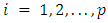 .The following assumptions are considered under model (1): a) stationarity, b)
  is a K-dimensional white noise process with
  is a fixed
  vector of intercept terms allowing for the possibility of a non-zero mean,
  , and c)
  is time invariant with positive definite covariance matrix.The Dickey Fuller (DF) test is used to test for unit root in first order autoregressive model, AR (1), with the basic assumption that errors are white noise. The Phillips-Perron (PP) test is an extension of the DF tests to ensure serial correlation in the errors terms by including more lag difference terms of the dependent variable. Besides this, the PP
  –statistic is used to identify whether it requires differencing a time series data or not to make it stationary with the various cases of the test equations; say, to put a time trend in the regression model to correct for the variables deterministic trend.
  | (2) |
 and without trend
  and with intercept
  and without intercept
  .In each case, the testing procedure is based on
  , the null hypothesis of the PP
  –test is
  (unit root/ non-stationarity or the data needs to be differenced to make it stationary) against the alternative
  (the data is stationarity and doesn’t need to be differenced). The other stationarity tests developed by Kwiatkowski, Phillips, Schmidt and Shin (KPSS) (1992), is different from the PP unit root test. In PP (Phillips Perron) tests the null hypothesis is unit root against the alternative hypothesis of stationarity. On the other hand, Charemza and Syczewska (1998), Maddala and Kim (1998) proposed that it should be tested where the null hypothesis is that of the stationarity against the alternative hypothesis of a unit root. The key idea behind such tests has been to look for a substantiation of the evidence suggested by standard PP tests. KPSS is mainly based on LM type test, in which the null hypothesis which states stationarity is stated against the alternative hypothesis of unit root (non-stationarity), Muhammad (2012).
 2.2.1. Determining the VAR Order
- If
 is a
is a  process, as to Equation (1), it is useful to fit a
  model to the available multiple time series with
  . In other words, if
  is a
is a  process, in this sense it is also a
  process. Therefore, call
  a
a  process if
  for
for  and
and  for
for  so that
  is the smallest possible order. This unique number will be called the VAR order. The other most popular method to choose the lag order
  is to use information criteria. An information criterion is designed to consistently find the model that fits better the data from a group of models. The decision about how many lag order to be included in the regression depends upon the model selection criterion, that is determined by minimizing the Schwartz Bayesian Information Criterion (BIC) or minimizing the Akaike Information Criterion (AIC) or lags are dropped until the last lag is statistically significant.
 There are three different criteria that are used to choose the order
  . Each one may choose different models. They differ by the penalization from the inclusion of additional parameters:
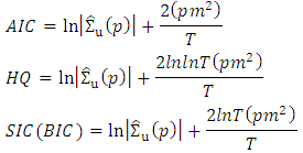 The penalization is such that
 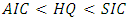 . This implies that the SIC (Schwarz IC or Bayesian IC) generally chooses models with a smaller
  while AIC (Akaike) chooses models with a higher order
  .
.2.2.2. Co-integration Test
- The application of unit root tests discussed in the previous sub-sections may not provide a conclusive result regarding the order of integration of the variables of interest. Thus, after the assessment of stationarity of the variables it is important to look at the order of integration before discussing about short and long-term relation of variables. The two common tests for co- integration are the Engle and Granger (1987) two-steps procedure and the Johansen (1991) maximum likelihood procedure. The determination of the number of co-integrating vectors is usually based on the method of two likelihood ratio (LR) test statistics; the trace test and the maximum eigenvalue test. These methods allow us to test the existence of long-term relationship between the dependent and the explanatory variables in a multivariate framework. In this study we used both tests.
2.2.3. Estimation
- The most popular method to choose the lag order
 is to use information criteria. An information criterion is designed to consistently find the model that fits better the data from a group of models. The decision about how many lag order to be included in the regression depends upon the model selection criterion, that is determined by minimizing the Schwartz Bayesian Information Criterion (BIC) or minimizing the Akaike Information Criterion (AIC) or lags are dropped until the last lag is statistically significant.For a given sample of the endogenous variables
  and sufficient pre-sample values
  , the coefficients of a VAR(p)-process can be estimated efficiently by least-squares applied separately to each of the equations. Because the disturbances are assumed to be normally distributed, the conditional density is multivariate normal distributed (Sims (1980); Lutkepohl (1999); Watson (1994)):
 The conditional density of the
  observation is:
 The likelihood function is the product of each one of these densities for
  . The log-likelihood function is the sum of the log of all these densities and thus it becomes:
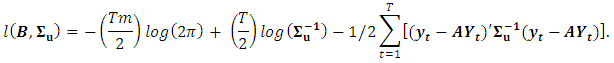 The estimated
  , which maximizes the log-likelihood is the ML estimator of the VAR coefficients:
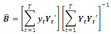 This means that the ML estimator of the VAR coefficients is equivalent to the OLS estimator of
  on
on  which is equivalent to the system multivariate estimator.The ML estimator for the variance is:
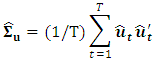 where,
 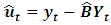 .The ML estimator of the variance is consistent, but it is biased in small samples, so it is common to use the variance estimator adjusted by the number of degrees of freedom:
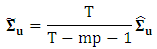 The (asymptotic) distribution of the coefficients of the
  equation of the VAR model is:
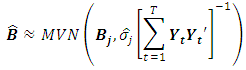 where,
  , that is, the coefficients’ variance can be computed using equation-by-equation OLS estimation. Because the coefficients are asymptotically normal, significance tests for each coefficient can be applied by comparing the t-statistic with the normal distribution.The estimated values maximize the log-likelihood function and are the ML estimators of the VAR coefficients. Because the coefficients are asymptotically normal, significance tests for each coefficient can be applied by comparing the t-statistic with the normal distribution. The Wald statistics can be employed to test hypothesis that impose restrictions on the coefficients.
2.2.4. Granger Causality Test
- In economics, systematic testing and determination of causal directions only became possible after an operational framework was developed by Granger (1969) and Sims (1972). The most widely used operational definition of causality is the Granger definition of causality, crucially based on the axiom that the past and present may cause the future but the future cannot cause the past (Granger and R. Joyeux, 1980). The structure of the VAR model provides information about a variable’s or a group of variables’ forecasting ability for other variables. According to the Granger causality approach a variable
 is caused by
  , if
, if  can be predicted better from past values of
  and
and  than from past values of
  alone. For a simple bivariate model, the pattern of causality can be identified by estimating regression of
  and
and  on all the relevant variables including the current and past values of
  and
and  and by testing the appropriate hypothesis. By using the following model the causality between variables can be tested.Two causality tests are implemented. The first is a F-type Granger-causality test and the second is a Wald-type test that is characterized by testing for nonzero correlation between the error processes of the cause and effect variables. For both tests the vector of endogenous variables yt is split into two sub-vectors
  and
and  with dimensions
  and
and  with
with  . For the rewritten VAR(p):
 | (3) |
 does not Granger-cause
  , is defined as
  for
for  . The alternative is:
  for
for  . The test statistic is distributed as
  with
with  equal to the total number of parameters in the above VAR(p) (including deterministic regressors).The null hypothesis for instantaneous causality is defined as:
  , where
  is a
is a  matrix of rank
  selecting the relevant co-variances of
  and
and  ;
;  . The Wald statistic is defined as:
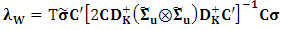 | (4) |
 with
with  .K and
  . The duplication matrix
  has dimension
  and is defined such that for any symmetric
  matrix A,
  holds. The test statistic
  is asymptotically distributed as
  .
.2.3. Forecasting
- As forecasting is one of the main objectives of multiple time series analysis forecasts for horizons
 of an empirical VAR(p)-process can be generated recursively according to Box and Jenkins (2008).
 where,
  for
for  .
. The matrices
  are the empirical coefficient matrices of the Wald moving average representation of a stable VAR(p)-process and the operator
  is the Kronecker product.
2.3.1. Impulse Response Function and Variance Decomposition
- Further, we might be interested in causal inference, forecasting and diagnosis of the empirical model's dynamic behavior, i.e., impulse response functions (henceforth: IRF) and forecast error variance decomposition (henceforth: FEVD). Impulse Response FunctionThe impulse response test shows the effects of an exogenous shock on the whole process over time (Stock, and Watson, 1990). The idea is initially to look at the adjustment of the endogenous variables and to detect the dynamic relationships among contemporaneous values of the variables over time, after a hypothetical shock in time t. This adjustment is compared with the time series process without a shock, i.e. the actual process. The impulse response sequences plot the difference between this two time paths which offers additional arguments for adjusting its appearance. The Wolds moving average decomposition for stable VAR(p)-process which is defined as:
 with
with  and
and  Thus, it is possible to pre-occupy the effect of a non-recurring shock in one variable, to all variables over time. The positive definite symmetric matrix
  can be written as the product
  , where
  is a lower triangular non-singular matrix with positive diagonal elements. Thus, one could summarize the result in any covariance stationary VAR(p) process as a Wolds representation by using the method of Ender (1995) of the form:
 | (5) |
 and
and  is white noise with covariance matrix
  with,
with,  is a vector moving average process and
  are the weight of past shocks are determined recursively using
 where
where  and
and  for
for  as in equation (1) of VAR(p) model specification.Once a recursive ordering has been established, the Wolds representation of
  based on the orthogonal errors
  is given as shown in (5) by:
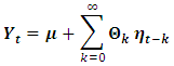
 is a lower triangular matrix. The impulse responses to the orthogonal shocks
  are
are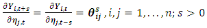 | (6) |
 is the
  term of
  .A plot of
  against s is called the orthogonal impulse response function (IRF) of
  with respect to
  . With n variables there are
  possible impulse response functions.Variance DecompositionAn alternative of impulse responses, to receive a compact overview of the dynamic structures of VAR models, are variance decomposition sequences. The VDCs show the portion of the variance in the forecast error for each variable due to innovations to all variables in the system (Enders, 1995). This method is also based on a vector moving average model and orthogonal error terms. In contrast to impulse response, the task of variance decomposition is to achieve information about the forecast ability. The idea is that even a perfect model involves ambiguity about the realization of
  because of uncertainty in the error terms association. According to the interactions between the equations, the uncertainty is transformed to all equations. The aim of VDC is to reduce the uncertainty in one equation to the variance of error terms in all equations.The forecast error variance decomposition is based upon the orthogonalised impulse response coefficient matrices
  and allow the user to analyze the contribution of variable j to the h-step forecast error variance of variable i. If the orthogonalised impulse reponses are divided by the variance of the forecast error
  , the resultant is a percentage figure. Formally:
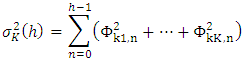 which can be written as:
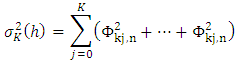 Dividing the term
  by
by  yields the forecast error variance decompositions in percentage terms.
3. Results and Discussion
3.1. Descriptive Measures
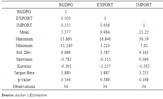
- This study aimed at examining the relationship between three macroeconomic indicator variables, namely: real economic growth (RGDPG) measured as the rate of change of real GDP, exports of goods and services as percent of GDP (EXP) and import of goods and services as percent of GDP (IMP) of Ethiopian. A preliminary data analysis is conducted by displaying the summary statistics of the series involved as well as the corresponding time series plots (see Figure 1 (Appendix).The descriptive statistics displayed in Table 1 (Appendix) shows economic growth increased from its minimum value of -11.14 in 1985 to its maximum value 13.86 in 1987 as the rate of change of real GDP. The disparity of RGDPG about its mean was with standard deviation of 6.689. Both Export and import of goods and services as percent of GDP increased from their minimum values of 3.21 and 7.62 in 1992 respectively to their maximum values 16.84 and 36.59 in 2012 and 2006, respectively. There is medium and positive correlation of both export and import of goods and services to economic growth of Ethiopia. Export and import of goods and services are high and positively correlated in the study period. Skewness and kurtosis test values show that none of the variables is symmetric and mesokurtic. The Jarque Bera statistic is also calculated to check for normality. The null hypothesis of normal distribution for all variables is not rejected at 5% significance level.The time series plots of all series showed a long-term increasing trend indicating that they are related over the study period. The result also indicates the existence of some kind of non-stationarity and possibly non-linearity in the observed data series. For this purpose, the test is analyzed with constant and linear trend to gain power against trend stationarity results on level of variables.
3.2. VAR Model Fitting
3.2.1. Unit Root Test
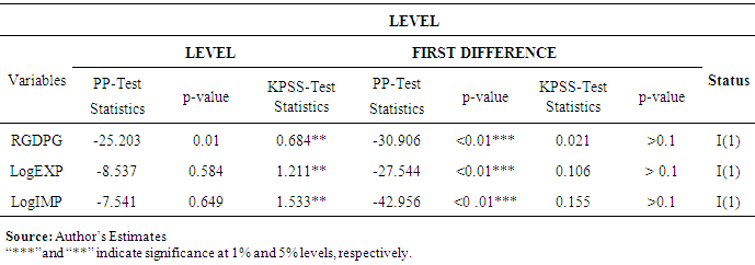
- In a next step, the we conducted unit root tests by applying the PP and KPSS tests regressions to the series. In model fitting procedure, conducting unit root test is important for checking stationarity of each data series as a non-stationary time series may produce spurious regression (Philips, 1986). Since the time series plot at level of each data series suggested a trend and potentially slow-turning around a trend line, we can assume that the equation has an intercept term and a time trend. PP and KPSS tests on all variables entered as logarithm except real economic growth for the set of data series with trend and first difference without trend, as reported in Table 2 (Appendix), indicate that all data sets are non-stationary at level, and attain stationarity after the first difference. Both tests provide strong evidence of non-stationarity at level, because PP failed to reject the null hypothesis while KPSS rejected the null hypothesis.The unit root test confirms that each time series is stationary at its first difference at chosen level of significance of 5%, that is, each time series is integrated of order one. Thus, for the essence of other subsequent tests, all the considered macroeconomic time series variables are regarded to be stationary at first difference integrated of order one i.e. I(1).
3.2.2. Determining Lag Order
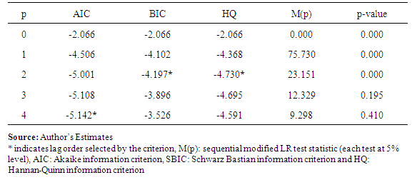
- The optimal lag-length of the lagged differences of the tested variable is determined by minimizing the Akaike Information Criteria (AIC) and Schwarz Bastian Information Criteria (BIC). Johansen and Juselius start by determining the co-integration rank. Because inferences on the co-integration space spanned by its vectors are dependent on whether or not linear trends exist in the data. Assuming that the data series of the three macroeconomic variables follow a VAR model, we applied the information criteria to specify the order. The AIC criteria select a VAR(4) while BIC and HQ criteria select a VAR(2) model as shown in Table 3 (Appendix), and thus the joint optimum lag length of order two was considered.
3.2.3. Co-integration Test
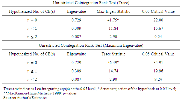
- The application of unit root tests discussed in the previous sub-sections may not provide a conclusive result regarding the order of integration of the variables of interest. Thus, after the assessment of stationarity of the variables: RGDPG, LogEXP and LogIMP (see Table 2 in Appendix), it is important to look at the order of integration before discussing about short and long-term relation of variables. The two common tests for co-integration are the Engle and Granger (1987) two-steps procedure and the Johansen (1991) maximum likelihood procedure. The determination of the number of co-integrating vectors is usually based on the method of two likelihood ratio (LR) test statistics; the trace test and the maximum eigenvalue test. These methods allow us to test the existence of long-term relationship between the dependent and the explanatory variables in a multivariate framework. In this study we used both tests.Pre-assumption, the individual components of
 are at most I(1) variables. Since both real exchange rate and interest rate exhibit an upward drift, the constant vector of the data is not 0. The study adopted cointegration test to examine whether the four variables under study had long-term equilibrium relationship. We calculate the trace statistics trace
  and the maximum eigenvalue statistics
  with null hypotheses of
  and
and  versus alternatives
  and
and  , respectively.The values of the test statistics and critical values (at 5% level tests) are listed in Tables 4 (Appendix) corresponding to the eigenvalues. The null hypothesis is rejected when the test statistic exceeds the critical level. Accordingly, With p = 0 the co-integration tests findings indicated that both trace test and max eigenvalue static are significant at 5% level. Thus, the Johansen cointegration test suggests that there is no long run relationship between export and import of goods services and economic growth in case of Ethiopia. This implies
  is not co-integrated. So that
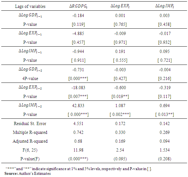
  follows a VAR(2) model. Thus we fitted VAR(2) to the stationary differenced data series and conducted diagnostic tests with respect to the residuals.The focus of this study was to assess the dependency of current values of economic variables: RGDPG, logEXP and logIMP on their own past as well as on the past values of other variables. Based on the above results, unrestricted VAR model with order of two was fitted and the results are presented in Table 5 (Appendix). In particular, the current real economic growth is negatively related to its own first two lags, to the first two lags of export and to first lag of import but positively related to second lag of import of goods and services. The current export of goods and services are negatively related to its own first two lags, but positively related to the first two lags of both the real economic growth and import of goods and services. Import of goods and services is positively related to its own second lag and first lags of real economic growth and negatively related to its own first lag, to the second lag of real economic growth and to the first two lags of export of goods and services. Based on the above discussion, results of unrestricted VAR model fitted with significant estimated coefficients of
 are presented in Equations (7)- (9) below, respectively (see also Table 5 in Appendix).
 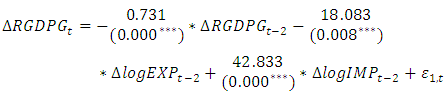 | (7) |
 | (8) |
 | (9) |
 , when considered as dependent variable, is reported in Equation (7). The estimated coefficients
 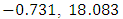 and
and  of
of  and
and  are highly significant at 5% significance level with p-values
 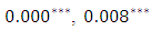 and
and  , respectively. The overall statistically significant negative coefficients of
  and
and  imply that the effect of a unit increase in total
  and
and  while keeping other factors constant results in reduction of 0.73% and 18.08% of current total
  , respectively. The statistically significant positive coefficients of
  imply that the effect of a unit increase in total
  while keeping other factors constant results in 48.83% increment of current total real economic growth of Ethiopia. According to the result of the fitted VAR model, in addition to its own two years lag effect of real economic growth, a significant impact of export and import of goods and services in the past two years lag on current economic growth is detected in the study period. This shows that real economic growth of Ethiopia has a significant dynamic relationship with both export and import during the study period. The Adjusted R-square value for this model is 0.68, indicating that 68% of the variation in the future
  observation is explained, and shows a medium predictive power with
 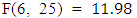 ,
,  and
and  .Similarly, in Equations (8) when
  is considered as dependent variables, it can be concluded that in while a two years lagged value of export of goods and services,
  , have own negative significant effect of 0.60, with p-value of
  ,
,  included in the model has a significant positive effect on export in their second lags. This shows that the current export of goods and services has a dynamic relationship with two years lag of import of goods and services in Ethiopia during the study period. On the other hand, the past real economic growth has no effect on import of goods and services. The Adjusted R-square value for this fitted model is 0.1694 indicating that 17% of the variation in the future
  observation is explained, and shows a low predictive power with
  ,
,  and
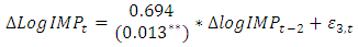
and  .As to the model in Equations (9) Economic growth in Ethiopia in the past doesn’t have a significant impact on current import of goods and services and vice versa. Furthermore export didn’t significantly affect import, while own past two years lag of import of goods and services considerably affect current import of goods and services during the study period. The Adjusted R-square value for this model is 0.094 indicating that 9% of the variation in the future
  observation is explained, and shows a very low predictive power with F (6, 25) = 1.534, P-value(F) = 0.208 and n=31. Finally, its roots are checked for model stability, the eigenvalues of the companion form are
  = (0.774, 0.774, 0.533, 0.533, 0.494, 0.328) all less than one. It signifies that the VAR model fitted to the data set is stable.
3.2.4. Diagnostic Checking
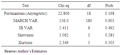
- Once a VAR-model has been estimated, it is of pivotal interest to see whether the residuals obey the model’s assumptions. That is, we should check for the absence of serial correlation and heteroscedasticity and see if the error process is normally distributed. The Breusch-Godfrey test for serial correlation with p-values less than 5% indicate the presence of serial correlation. The non-rejection of the null hypothesis of no heteroscedasticity in case of multivariate ARCH (MARCH) test with p-values less than 5% indicate the presence of heteroscedasticity. A further characterization of our model includes VAR residual normality test using the Orthogonal Cholesky test method for the null hypothesis: H0: residuals are multivariate normal with p-values less than 5% indicate non-normality.Results in Table 6 (Appendix) indicate the non-rejection of the null hypothesis of no serial correlation in case of LM test, no heteroscedasticity in case of MARCH test and residuals are multivariate normal at 5% level of significance. Thus the results confirm that the residual terms are pure white noise, i.e. they are well behaved and the null hypothesis of no serial correlation, no heteroscedasticity and residuals are multivariate normal are not rejected as shown by the insignificant Chi-square values.As it can be observed in Figure 2 (Appendix), the series from VAR residuals presents a feature specific to non-linear models, namely volatility clustering. Thus, the non-linear dependencies can be explained by the presence of conditional heteroscedasticity. This may be handled in study of conditional volatility modelling, like multivariate GARCH models.In general, the robustness of the model was confirmed by various diagnostic tests: MARCH test; Jaque-Berra normality test, LM serial correlation test. The diagnostic tests result in Table 6 also revealed that the model is adequate and has the desired econometric properties, i.e. has correct functional form, its residuals are serially uncorrelated and homoscedastic and multivariate normal.
3.2.5. Granger Causality Tests
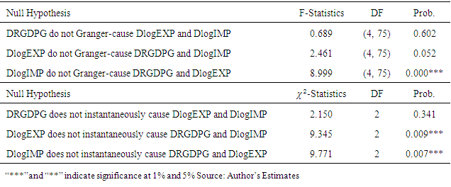
- In this section we apply Granger causality tests on the first difference of LogGDP, LogEXP and LogIMP to determine the pair-wise causal relationship among them. This procedure is particularly attractive over the standard VAR because it permits temporary causality to emerge from the lagged coefficients of the explanatory differenced variable. It systematically tests for nonzero correlation between the error processes of the cause and effect variables. However, the reliability of results of the Granger causality test depends on stationarity of the variables. For the variables considered in this study the unit root test reported in Table 1 suggests stationarity of each variable at first difference. The very low p-values in both types of causality tests (Granger and instantaneous) we reject non-causality, supporting possible causation. We have determined a causal relation, because there are macroeconomic reasons to believe in a causal relation is at all plausible.The results of multivariate Granger causality tests reported in Table 7 (Appendix) signify the existence of a significant and a strong uni-directional causality from import of goods and services to both real economic growth and export of goods and services with F-test statistic of 8.999 at 4 and 75 degrees of freedom with p-value of
 . On the other hands, we fail to accept the Granger causality from real economic growth to exports and import of goods and services of Ethiopia in the study period.Table 7 in the bottom panel also reports the Wald test statistic for multivariate instantaneous causality tests which is asymptotically Chi-square obtained together with the estimate p-values. The null hypothesis export does not instantaneously cause real economic growth and import as well as import does not instantaneously cause real economic growth and export are both rejected at 5% significance level with p-values
  and
and  , respectively. Similar to the Granger causality test above, we fail to accept the instantaneous causality from real economic growth to exports and import of goods and services of Ethiopia in the study period.In summary, the study found statistically sound evidence to conclude that there was no direct causality from export of goods and services to current real economic growth of Ethiopia as measured by GDP, whereas import of goods and services significantly affects and Granger causes both economic growth and export of goods and services. It is interesting since according to the import-led growth theory, imported raw materials should be used in the goods to be exported, which in turn promote the economic growth. The presence of a causal link between export and growth has implications of great consequence on development strategies for developing countries (Wadad Saad, 2012). If export causes economic growth, then the achievement of a certain degree of development may be a prerequisite for the country to expand its exports. Thus, exports were important in fueling economic growth of Ethiopia for the whole study period (1982-2015).
3.3. Forecasting
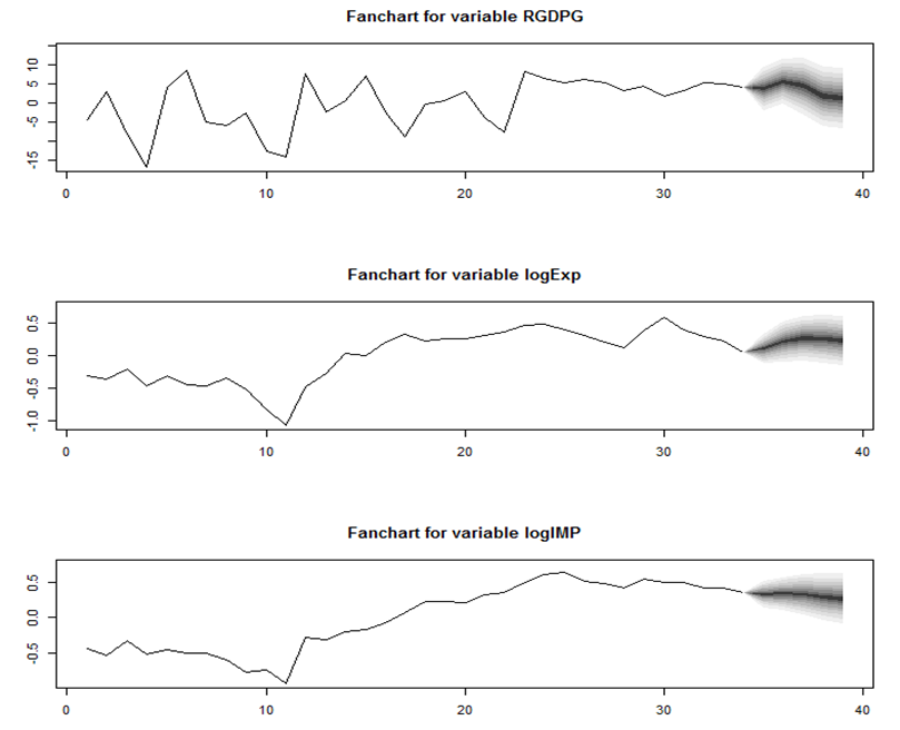
- Once a VAR-model has been estimated and passes the diagnostic tests, it can be used for forecasting. Indeed, one of the primary purposes of VAR analysis is the detection of the dynamic interaction between the variables included in a VAR(p)-model. Aside from forecasts, other tools for investigating these relationships are impulse response analysis and forecast error variance decomposition. The out-of-sample forecasting activity is obviously important in time series analysis and VAR models are no exception. It simply plugs in the past values recursively to get subsequent (future) values. It also provides a confidence interval around the forecasts.Figure 3 (Appendix) shows the forecasts produced from the VAR(2) fitted above. At the beginning of the forecast horizon the RGDPG is growing slowly and decline around the last forecasting horizons. While export of goods and services was predicted to growing sharply throughout forecast horizons, import of goods and services was predicted to decrease slowly in the throughout the predicted time horizons. This may be due to the fact that Ethiopia is working hard towards transforming its economy through agricultural development led industrialization strategy that promote export rather than import of manufactured goods.Results of Impulse Response AnalysisThe impulse-response functions trace the effects of a one-time shock to one of the innovations on current and future values of the endogenous variable. It also allows us to establish the length of time it takes for the effects of shocks to die out and approximate the effects of an exogenous dynamic shock among residuals on the whole process of the endogenous variable over time.Impulse response estimates from our vector auto-regression model indicate that, from the top row of Figure 4 (Appendix) we observe that one positive shock to RGDPG leads to negative response from exports in the lower lags, which dies out in period 4, while the shock to RGDPG from imports produces continuous responses. In the middle row of the same figure, a positive shock to exports lead to a positive response from RGDPG and import and they die out in period 4. In addition, positive shocks to imports lead to a positive response from RGDPG and exports and die out in period 4 and 5, respectively, as shown in bottom row of Figure 3A (Appendix). This supports the previous argument of imports’ play a significant role on Ethiopia’s real economic growth during 1982-2015. While the strong relationship between RGDP growth and exports is in the case of Ethiopia is due to an increase in exports.Results of Variance Decomposition Analysis The relative importance of shocks can be analyzed through variance decomposition, which tells us the proportion of the variation in the variable that is from its own shocks and due to the shocks in other variables (Enders, 2010). Variance decomposition measures the percentage of the forecast error variances at various forecast horizons that are attributable to each of individual shocks. Such procedure allows one to see the long-run percentage variation in a variable as a result of shocks to other variables. If the share of variation of a variable would be 0%, then that variable would be completely exogenous in the model as explained in Enders (1995).Results in Figure 5 (Appendix) illustrate the results of forecast error variance decomposition of fitted VAR(2) model using recursive causal ordering RGDPG, logEXP, logIMP. The first row gives the variance decomposition for RGDPG. At short horizons, most of the variance is attributable to own shocks but at long horizons import of goods and services shocks accounts for almost half the variance. The second row gives the variance decomposition for logEXP and shows that in the short horizons most of the variances of the forecast error is due to own shocks, but in the long horizons import of goods and services shocks account almost 30% of the variation. The third row gives the variance decomposition for logIMP. In the short time horizons, 54% of the variance is due to own shocks, 38.6% of the variance is accounted shocks from export of goods and services, but at long horizons variance is due to own shocks increase to 63% and that of export of goods and services decrease to almost 30% of the variance. The rest a small fraction of variance is accounted due to real economic growth shocks.In general, variation in export and import has played the most important role in explaining the dynamic changes in real economic growth next to its own variation. Therefore, the result signifies that no variable would be completely exogenous in the model. Additionally, FEVD result revealed that the growth of import is the most important macroeconomic variables that account for the innovation in real economic growth in Ethiopia in the long term which is also confirm to the results of VAR analysis above. Lastly, the IRFs and FEVDs computed above depend on the imposed recursive causal ordering. However, the ordering of the variables have a little effect on the IRFs and FEVDs because the errors in the reduced form VAR are nearly uncorrelated.
4. Conclusions
- The driving objective of this study has been to investigate the nature of the relationship of macroeconomic variables, namely export and import of goods and services, and real economic growth in the context of Ethiopia. We tested if whether exports, imports and real GDP growth are cointegrated using Johansson approach and the test suggests that there is no long run relationship between export and import of goods services and economic growth in case of Ethiopia. Time series econometric techniques: The VAR model infers that the current real economic growth of Ethiopia measured as rate of real GDP is significantly affected by past two lagged values of its own, export and import of goods and services. The effect is negative for lags of export and its own lags and positive for import. Similarly, the current export is also negatively affected by its own past two lagged values, while positively affected by past values of import of goods and services. Import is negatively affected by its own past two lagged values only.From empirical results of Granger causality test, the study found statistically sound evidence to conclude that there was no direct causality from export of goods and services to current real economic growth of Ethiopia as measured by rate of real GDP, whereas import of goods and services significantly Granger causes both real economic growth and export of goods and services. Empirical results of impulse response function analysis show that shock to RGDPG leads to negative response from exports which dies out after five years, while the shock to RGDPG from import of goods and services produces continuous responses. The result also signifies that Ethiopian economic growth highly benefits from export performance because of the feasibility of export-led growth scenario in Ethiopia and promotes foreign exchange rate. Therefore, Ethiopia can enhance its economic growth by improving the competiveness of its export items.The forecast error variance decomposition (FEVD) test results indicate that most of the variance in each variable is attributable to own shocks but at long horizons import of goods and services shocks accounts almost half of variance of real economic growth. The analysis also shows that shocks to imports of goods and services lead to a significant response in real economic growth. On the other hand, shocks to exports have a low response on real economic growth, supporting the weak relationship between real economic growth and exports for the case of Ethiopia.Since, Ethiopia is working hard towards transforming its economy through agricultural development led industrialization strategy; it is recommended that sustainable economic growth could be achieved by attracting additional capital investment to the country with enhanced technology and industrial production for export. Thus development strategies based on Export-Led Growth (ELG) hypothesis could be appropriate for Ethiopia.
Appendix
|
|
|
|
|
|
|
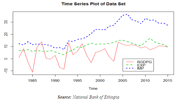 | Figure 1. Time Plot for GDP, Import and Export |
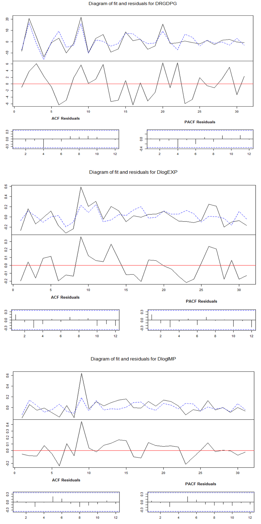 | Figure 2. Plot of Fitted VAR(2) and Residual Analysis for 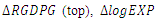 (middle) and (middle) and  (bottom) (bottom) |
 | Figure 3. Forecasting plots of a fitted VAR Model for the Yearly Economic Growth (top), Yearly Export of Goods and Services (middle) and Import of Goods and Services (middle). The forecasts are for the Logarithm of Observed series and the forecast origin is 2015 |
 | Figure 4. Impulse Response Function using Recursive Causal Ordering RGDPG, logEXP, logIMP |
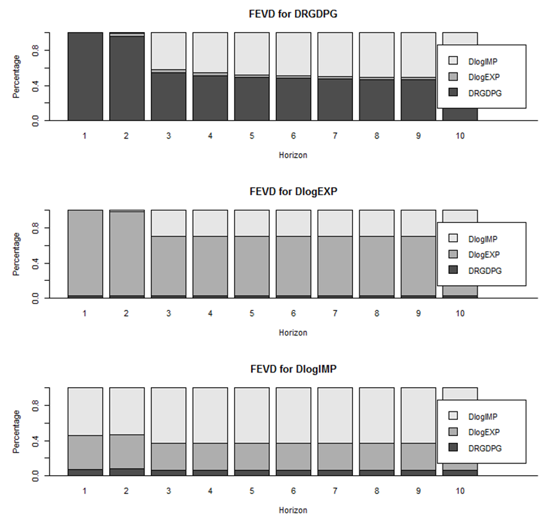 | Figure 5. FEVDs depend on the imposed recursive causal ordering  |