-
Paper Information
- Next Paper
- Paper Submission
-
Journal Information
- About This Journal
- Editorial Board
- Current Issue
- Archive
- Author Guidelines
- Contact Us
American Journal of Economics
p-ISSN: 2166-4951 e-ISSN: 2166-496X
2016; 6(6): 281-299
doi:10.5923/j.economics.20160606.01

Modelling Volatility and the Risk-Return Relationship of some Stocks on the Ghana Stock Exchange
 Abstract
 Reference
 Full-Text PDF
 Full-text HTML
Abonongo John, Oduro F. T., Ackora-Prah J.
College of Science, Department of Mathematics, Kwame Nkrumah University of Science and Technology, Kumasi, Ghana
Correspondence to: Abonongo John, College of Science, Department of Mathematics, Kwame Nkrumah University of Science and Technology, Kumasi, Ghana.
| Email: |  |
Copyright © 2016 Scientific & Academic Publishing. All Rights Reserved.
This work is licensed under the Creative Commons Attribution International License (CC BY).
http://creativecommons.org/licenses/by/4.0/

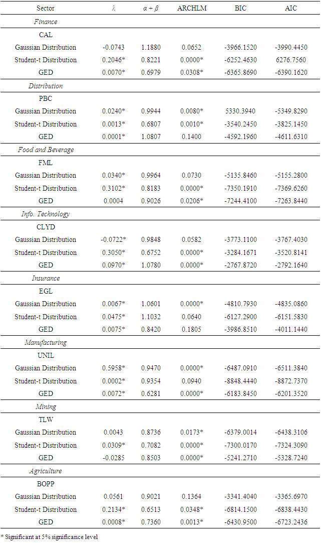
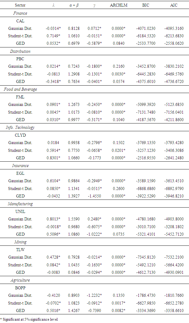
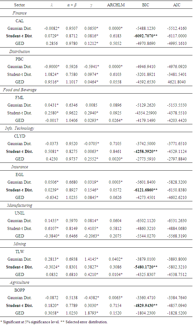
The volatility and the risk-return trade off of stocks or stock markets play essential role in investment decision making, financial stability among others. This paper modelled the volatility and the risk-return relationship of some stocks on the Ghana Stock Exchange using univariate GARCH-M (1,1) models with three distributional assumptions namely, the student-t, GED and Gaussian distributions. The results showed that, the market was bullish for investors of most of the stocks and that there was a high probability of gains than losses. All the stocks were extremely volatile. The results also indicated the existence of positive risk premium meaning investors were compensated for holding risky assets. The results also showed that, the asymmetry models gave a better fit than the symmetry model indicating the presence of leverage effect among the selected stocks. The TGARCH-M (1, 1) model with the student-t distribution was the appropriate model selected.
Keywords: Risk-return, Volatility, Stocks, Risk premium, GARCH-M
Cite this paper: Abonongo John, Oduro F. T., Ackora-Prah J., Modelling Volatility and the Risk-Return Relationship of some Stocks on the Ghana Stock Exchange, American Journal of Economics, Vol. 6 No. 6, 2016, pp. 281-299. doi: 10.5923/j.economics.20160606.01.
Article Outline
1. Introduction
- The stock market provides a framework within which capital formation takes place and where previously issued securities are traded among investors for productive investment. The Stock Exchange plays an integral role in the capital formation and wealth creation activities in any nation. One of the essential characteristics that need distinct consideration by any investor or policy maker is the volatility of stock returns. Volatility can be defined as a statistical measure of the dispersion of returns for a given security or market index and it can either be measured using the standard deviation or variance between returns from that same security or market index [23].[8] introduced the ARCH-M model by extending the ARCH model to allow the conditional variance to be determinant of the mean. Whereas in its standard form, ARCH model expresses the conditional variance as a linear function of past squared innovations, in this new model they hypothesized that, changing conditional variance directly affect the expected return on a portfolio. Their results from applying this model to three different data sets of bond yields are quite promising. Consequently, they concluded that risk premia are not time invariant; rather they vary systematically with agent’s perceptions of underlying uncertainty.[20] extended the ARCH framework in order to better describe the behaviour of return volatilities. Nelson’s study was important because of the fact that it extended the ARCH methodology in a new direction, breaking the rigidness of the G/ARCH specification. The most important contribution was to propose a model (Exponential Autoregressive Conditional Heteroskedasticity (EARCH)) to test the hypothesis that the variance of return was influenced differently by positive and negative excess returns. His study found that not only was the statement true, but also that excess returns were negatively related to stock market variance. [10] modified the primary restrictions of Generalized Autoregressive Conditional Heteroskedasticity- in Mean (GARCH-M) model based upon the truth that GARCH model enforce a symmetric response of volatility to positive and negative shocks, introduced the Glosten-Jagannathan-Runkle Generalized Autoregressive Conditional Heteroskedasticity (GJRGARCH) and the Threshold Generalized Autoregressive Conditional Heteroskedasticity (TGARCH) models. They conclude that there is a positive but significant relation between the conditional mean and conditional volatility of the excess return on stocks when the standard GARCH-M framework was used to model the stochastic volatility of stock returns.[6] also investigated the behaviour of stock return volatility of the Nigerian Stock Exchange (NSE) returns using GARCH (1, 1) and the GJR-GARCH (1,1) models assuming the Generalized Error Distribution (GED) using data from the monthly all share indices of the NSE from January 1999 to December 2008. He sought to do this by examining the NSE return series for evidence of volatility clustering, fat-tails distribution and leverage effects, because they provided essential information about the riskiness of assets on the market. He discovered that there exists volatility clustering on the Nigeria Stock Exchange (NSE) and used GARCH (1,1) to model that. He captured the existence of leverage effects in the series with the GJR- GARCH (1,1) model. The GED shape test also revealed a leptokurtic returns distribution. The entire results revealed that there was evidence of volatility persistence, fat-tail distribution, and leverage effects present in the NSE. He concluded that the volatility of the stock returns was persistent in Nigeria and that the shape parameter estimated from GED revealed evidence of leptokurtosis in the NSE returns distribution. In modelling the volatility on the Johannesburg Stock Exchange (JSE) employing ARCH-type models, [18] found that volatility was symmetric and was not a commonly priced factor. This result was obtained by considering two portfolios (with data from 1973 to 2002): the All Share Index (ALSI) and a portfolio with 42 stocks. The portfolio of 42 stocks was used because the ALSI is dominated by resource stocks and thus it was essential to have a portfolio that was not improperly influenced by the dynamics of the resource stocks. This result was echoed by [3], who primarily studied returns and volatility linkages between South Africa (SA) and the world major equity markets. Using a GARCH-M methodology to test the risk-premium hypothesis the authors, like [18], found that volatility is not a commonly priced factor and found that volatility is asymmetric.Using a GARCH-M model, [20] investigated stock market volatility in the East European emerging markets of Hungary and Poland. The study covered a period from 1994 to 1996 using daily data from the Bulgarian and Warsaw stock markets. A similar result was obtained by [27] using an extension to the GARCH model, the EGARCH model realized that, there was a significant positive risk-return relationship in Bahrain, Oman and Saudi Arabia, while in Egypt, Jordan, Morocco and Turkey volatility was not priced. Using the same model, [12] found evidence in support of a negative risk-return relationship on the Indian stock market using the S and P CNX (Console Energy Inc.) Nifty for the period 1990 to 2004. Similarly, using the EGARCH-M model [21] found that positive returns were matched with higher volatility on Pakistan’s stock exchange (Karachi stock exchange). [1] investigated the relationship between risk, return and volume on the Bilbao stock exchange (1916 to 1936) using the augmented GARCH-M model that was modified to account for volume traded. They found that there was little evidence of a significantly positive risk-return trade-off. [22] found a significant relationship between risk and return in 20 emerging markets. They further stated that the existence of such a relationship is highly dependent on the sample period used. They concluded that the difference between emerging and developed equity premiums follows a cyclical pattern that resembles the global business cycle.Also, using the GARCH, EGARCH, TGARCH and PGARCH models, [13] found a weak relationship between risk and return in the Macedonian Stock Exchange (MSE). The study used the MBI-10 index, which is the capitalization-weighted index consisting of up to 10 shares listed on the official market of the MSE, covering a period from 2005 to 2007. [13] tested the result assuming three different distributions; the Gaussian, Student-t and GED test and found that the TARCH model with a Student-t distribution was the best model to accurately model the data. [16] used a similar approach by using GARCH models with a Student-t and a Gaussian distributional assumption in investigating the risk-return relationship in the West African Economic and Monetary Union, using weekly returns for the period 1999 to 2005. The study revealed that, expected stock return has a positive but statistically insignificant relationship with expected volatility. He also found that volatility is higher during market booms than when the market declines.[25] studied the nature of stock market volatility and its relation to expected returns for ten industrialized countries (Australia, Belgium, Canada, France, Italy, Japan, Switzerland, the United Kingdom, the United States, West Germany). They used the GARCH-M specification and tested three different specifications for the conditional variance and expected market returns relationship, which are the linear, square root and log-linear specifications. The results of this study supported the findings of the preceding studies that did not find a significant relationship between conditional volatility and expected returns. [14] used a modified GARCH-M model in order to cater for skewness and kurtosis. The study used monthly US stock returns for the period from 1946 to 2002. They motivated this modification by arguing that the modified model was capable of modelling moderate skewness and kurtosis typically encountered in financial return series. The results of this study showed that there was a positive and significant relationship between risk and return. The essence of this paper is to model volatility and the risk-return relationship of some stocks on the Ghana Stock Exchange using univariate GARCH-M family of models assuming three distributional assumptions namely the Student-t, Generalized Error Distribution (GED) and the Gaussian distribution and under which distributional assumption the model performs best. This will provide investors and policy makers first-hand information about the nature of uncertainty on the Ghana Stock Exchange. That is, it will help investors in their investment decision making processes and assist regulators of the exchange to monitor and implement rules that will cause more companies to list on the exchange.
2. Materials and Methods of Analysis
2.1. Source of Data
- This paper employed secondary data of 8 equities (CAL Bank Limited, Produce Buying Company, Fan Milk Limited, Clydestone (Ghana) Limited, Enterprise Group Limited, Uniliver Ghana Limited, Tullow Oil Plc and Benso Oil Palm Plantation) from the Ghana Stock Exchange (GSE) and Annual Report Ghana databases comprising the daily closing prices from the period 02/01/2004 to 16/01/2015, totalling 7616observations.
2.2. Methods of Data Analysis
- The daily index series were converted into compound returns given by;
 | (1) |
 is the continuous compound returns at time
  ,
,  is the current closing stock price index at time
  and
and  is the previous closing stock price index.
 2.2.1. Unit Root Test: ADF Test
- The Augmented Dickey-Fuller (ADF) test was employed to determine whether the individual series studied have unit root or were covariance stationary. It was proposed [4] as an upgraded form of the Dickey-Fuller (DF) test. The ADF test assumes the hypothesis:
 (non-stationary) against
  (covariance stationary).where
  is the characteristics root of an AR polynomial and
  is an uncorrelated white noise series with zero mean and constant variance.The ADF test statistic is given by;
 | (2) |
 is the estimate of
  and
and  is the standard error of the least square estimate of
  . The null hypothesis is rejected if the
  significance level.
2.2.2. Jarque-Bera Test
- [11] is a goodness-of-fit test which examines if the sample data have kurtosis and skewness similar to a normal distribution.The test statistic is given by;
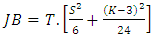 | (3) |
 If the sample data comes from a normal distribution JB should, asymptotically, have a chi-squared distribution with two degrees of freedom.
2.2.3. Univariate Ljung-Box Test
- The [17] was employed to test whether there exist autocorrelations
 in the returns series. The statistic is given by;
 | (4) |
 is the residual sample autocorrelation at lag l, T is the size of the series, k is the number of time lags included in the test.
  has an approximately chi-square distribution with k degree of freedom. The null hypothesis is rejected and concluded at α-level of significance that, the residuals are free from serial correlation when the p- value is greater than the significance.
2.2.4. Testing for ARCH Effects
- In applying GARCH methodology, it is very essential to examine the residuals for evidence of ARCH effects. The ARCH-LM test was employed. [15] documented that the Lagrange Multiplier (LM) test can be used to test the ARCH effect in a series. By representing the i lag autocorrelation of the squared or absolute returns by
 , the Ljung-Box statistic is given by;
 | (5) |
 The statistic of the LM test is given by;
 | (6) |
 is the number of restrictions placed on the model, T is the total observations and
  forms the regression.
 2.2.5. The Durbin-Watson Test
- [5] was employed to determine whether the error term in the mean equation follows an AR (1) process. The test requires the error term
 to be distributed
  for the statistic to have an exact distribution. The test statistic is given as;
 | (7) |
 and
and  and
and  are the observed and predicted values of the response variable for individual i respectively. d becomes smaller as the serial correlations increases.The hypothesis is given by;
 Also, the d statistic can take on values between 0 and 4 and under the null hypothesis d is equal 2. Values of d less than 2 suggest positive autocorrelation
  , whereas values of d greater than 2 suggest negative autocorrelation
  . When d is closer to 2, it suggest that there is no first order autocorrelation in the residuals.
2.2.6. The Breusch-Godfrey Test
- This is an LM test which is used to test for higher-order serial correlation in the disturbance.The test statistic is given by;
 | (8) |
 is the simple
  from the regression
 | (9) |
 The test is asymptotically
  distributed.
2.2.7. The Mean Equation
- In modelling volatility, it is very essential to specify an appropriate mean equation. The mean equation should be white noise series, that is it should have a finite mean and variance; constant mean and variance, zero autocovariance, except at lag zero. Comparatively following [24] and [3], this paper employed the mean equation given by:
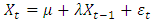 | (10) |
 is the returns for each equity in each sector,
  and
and  are constants and
  is the innovation.The Univariate GARCH-in Mean (GARCH-M) ModelMostly, the return of a security may depend on its volatility. In other for such a phenomenon to be modelled, there is the need to consider the GARCH-M model of [8].It is an extension of the basic GARCH model which allows the conditional mean of a sequence to depend on its conditional variance or standard deviation. The general form of the GARCH (p,q) model is given by;
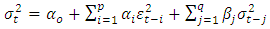 | (11) |
 and
and  and
and  is the squared volatility,
  is a constant,
  is the coefficient of the lagged squared residuals,
  is the lagged squared residual and
  is the coefficient for the GARCH component.The simplest GARCH-M model is the GARCH-M (1, 1) given by;
 | (12) |
 | (13) |
 and
and  are constants.
  is the returns on an equity or sector,
  is the squared volatility,
  is the coefficient of the standard deviation (risk premium parameter),
  is the coefficient of the lagged squared residuals,
  is the lagged squared residual from the mean equation and
  is the coefficient for the GARCH component (lagged conditional variance). To satisfy the stationary condition,
  .If
.If  is positive or negative and statistically significant, then increased risk given by an increase in conditional variance, leads to a rise or fall in the mean return, that is
  can be said to be time-varying risk premium. A statistically positive relationship will indicate that investors are compensated for assuming greater risk. But a negative relationship will indicate that investors react to factor(s) other than the standard deviation of equities from their historical mean.[8] also assumed that risk premium is an increasing function of the conditional variance of
  . That is, the greater the conditional variance of the return, the greater the compensation necessary to induce an investor to hold an asset for a long period [7]. This model will be tested for ARCH effects, and if the ARCH LM test reveals evidence of ARCH effects, the EGARCH-M will be employed.
2.2.8. The Exponential GARCH-M (EGARCH-M)
- This model captures asymmetric responses of time-varying variance to shocks and at the same time ensures the variance is always positive. It was developed by [20], the generalized form can be specified as EGARCH (p, q) given by;
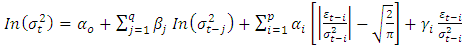 | (14) |
 is a constant,
  and
and  are the same as in GARCH-M and
  is the asymmetric response parameter (leverage parameter).If
  or there is arrival of good news, the total effect of
  is
is  ; if
; if  (arrival of bad news), the total effect of
  is
is  . The model is stationary and has a finite kurtosis if
  . That is there is no restriction on the leverage effect. There is no leverage effect if
  is negative.The sign of
  is expected to be positive in most empirical case so that a negative shock increases future volatility whereas a positive shock reduces the effect on future uncertainty. Also if
  and statistically significant, then negative shocks imply a higher next period conditional variance than positive shocks of the same magnitude.Assuming the mean equation in Equation (10), the simplest form of EGARCH-M is the EGARCH-M (1, 1), the variance equation is given by;
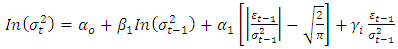 | (15) |
 , if volatility is asymmetric.In the original specification of the model, [20] assumed GED (Generalized Error Distribution) for the errors. If the distributional assumption of the errors are altered from the original, the model specification will leave the estimates the same except for
  . The TARCH-M will also be explored if the EGARCH-M does not fully eliminate the ARCH effects. Like the EGARCH-M model, the TARCH-M is an asymmetric model. However, the specification and interpretation differs from the EGARCH-M.
 2.2.9. The Threshold GARCH-M (TGARCH-M)
- This model was proposed by [10] and [27]. It is simply a respecification of the GARCH-M model with an additional term to account for asymmetry (leverage effect). In the general specification of this model, the TGARCH (p, q) model is given by;
 | (16) |
 is a constant, d is the asymmetric component and
  is the asymmetric coefficient.
  ,
,  and
and  are non-negative. Assuming the mean equation in equation (10), the variance equation for TGARCH-M (1, 1) is given by;
 | (17) |
 | (18) |
 , then leverage effects exist in stock markets and if
  then the impact of news is asymmetric [9]. Also when
  , the model collapses to the standard GARCH form. Nevertheless, when the shock is positive (good news), the volatility is
  , whereas if the news is negative (bad news), the effect on volatility is
  . Similarly, if
  is positive and statistically significant then negative shocks will have a larger effect on
  than positive shocks [2]. Also, since the conditional variance must be positive, the constraints of the parameters are
  and
and  . The model is stationary if
  .
.2.2.10. Distributional Assumptions of Error Term
- In GARCH model specification, it is more appropriate to consider the choice on the distributional assumption of the error term. Following [13], this study assumed three distributional assumptions; Student-t distribution, Generalized Error Distribution (GED) and Gaussian (Normal) distribution in order to account for fat tails that are common in most financial data. The ARCH models are estimated using the maximum likelihood approach given a distributional assumption. The contribution to the likelihood for observation t for the Student-t distribution is given by;
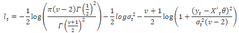 | (19) |
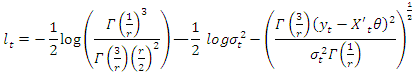 | (20) |
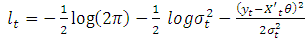 | (21) |
2.2.11. Model Selection Criterion
- This study employed two information criteria namely, Akaike Information Criterion (AIC) and Bayesian Information Criterion (BIC) in selecting the best model. Their respective estimations are given by;
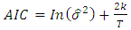 | (22) |
 | (23) |
 is the variance of the residuals,
  is the sample size, k is the total number parameters. For a GARCH (p,q) model,
  . The best model is the model that has least AIC, SBIC and HQIC values.
2.2.12. Model Diagnostic
- It is very essential to perform a diagnostic checks on the model after determining the best model and its corresponding distribution for the error term so as to establish whether the model and distribution are correctly specified. This study will employ the Ljung-Box test and Lagrange Multiplier (LM) test to test for the presence of autocorrelation and ARCH effects. The presence of autocorrelation and ARCH effects for both the raw series and the standardized residuals of the selected model will be tested.
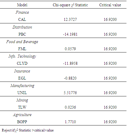
2.2.13. Cross Validation of GARCH-M (1,1) Family of Models
- The fitted model was cross validated with an out-sample forecast from 5th January, 2015 to 16th January, 2015. The chi-square goodness of fit test was employed. This is a statistical test that examines the level to which a set of observed sample data deviates from the corresponding set of expected values of the sample. The test statistic is given by;
 | (24) |
 is the observed returns series and
  is the expected returns series.
3. Results and Discussion
3.1. Descriptive Statistics
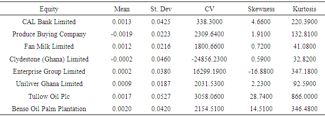
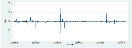
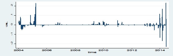
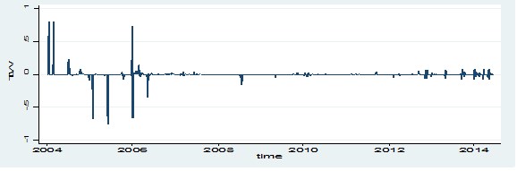
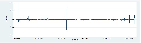
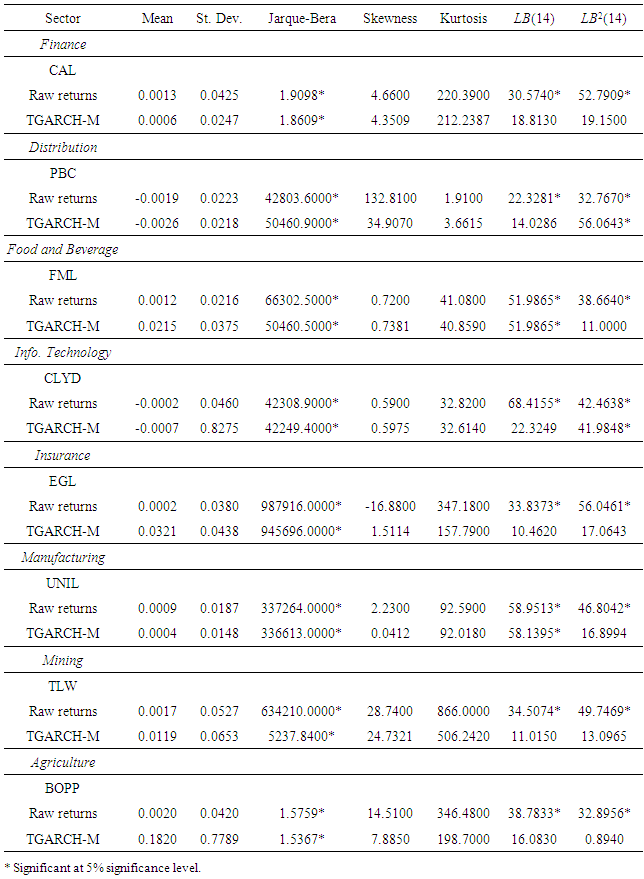
- The summary statistics of the returns series as reported in Table 1 reveals that most of the equities had positive mean returns ranging from 0.0002 to 0.0020 and negative mean returns ranging from -0.0019 to -0.0002. The highest mean return was recorded in Benso Oil Palm Plantation and the lowest mean return recorded in Produce Buying Company. A positive mean return indicates that investors of such equities made gains whereas those with negative mean return shows that investors made losses. The standard deviation as a measure of risk was high in Tullow Oil Plc (0.0527) and low in Uniliver Ghana Limited (0.0187) indicating the risk levels across the equities. The variability between risk and return as a measure of coefficient of variation ranges from -24856.2300 (Clydestone (Ghana) Limited) to 16299.1900 (Enterprise Group Limited). Also, most of the mean returns were positively skewed ranging from 0.5900 to 28.7400. This indicates that, the upper tail of the distribution of the return were ticker than the lower tail and that there were higher chances of gains than losses. That is, there was greater probability of making gains by investors in such equities. Nevertheless, Enterprise Group Limited recorded a negative skewness (-16.8800) indicating that there was a high probability of making loss than gain by investors. The excess kurtosis ranged from 32.8200 to 866.0000 which are greater than 3. This means that the underlying distribution of the returns leptokurtic in nature and heavy tailed and that there was more frequently extremely large deviations from the mean returns than a Normal distribution making the equities highly volatile.
|
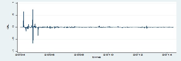 | Figure 1. Time Series plot of CAL Bank Limited Returns Series |
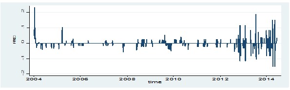 | Figure 2. Time Series plot of Produce Buying Company Returns Series |
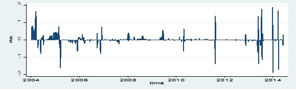 | Figure 3. Time Series plot of Fan Milk Limited Returns Series |
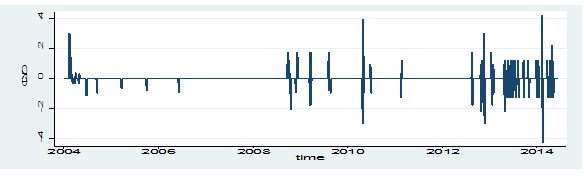 | Figure 4. Time Series Plot of Clydestone (Ghana) Limited Returns Series |
 | Figure 5. Time Series Plot of Enterprise Group Limited Returns Series |
 | Figure 6. Time Series plot of Uniliver Ghana Limited Returns Series |
 | Figure 7. Time Series plot of Tullow Oil Plc Returns Series |
 | Figure 8. Time Series plot of Benso Oil Palm Plantation Returns Series |
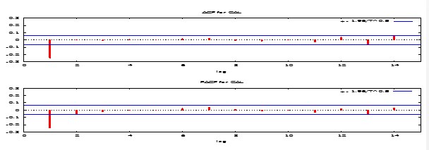 | Figure 9. ACF and PACF plot of CAL Bank Limited Returns Series |
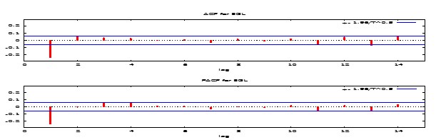
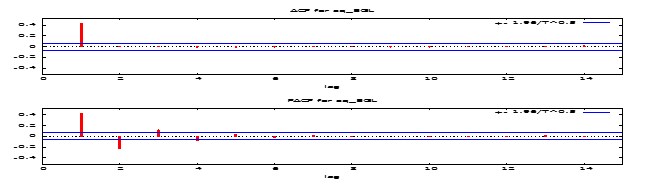
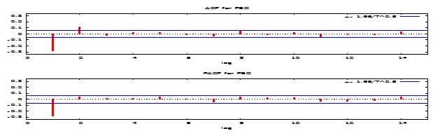 | Figure 10. ACF and PACF plot of Produce Buying Company Returns Series |
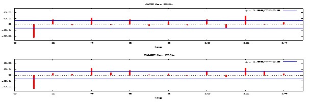 | Figure 11. ACF and PACF plot of Fan Milk Limited Returns Series |
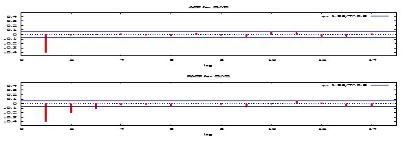 | Figure 12. ACF and PACF plot of Clydestone (Ghana) Limited Returns Series |
 | Figure 13. ACF and PACF plot of Enterprise Group Limited Returns Series |
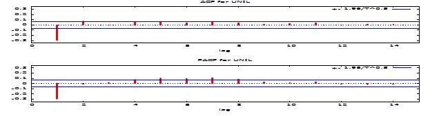 | Figure 14. ACF and PACF plot of Uniliver Ghana Limited Returns Series |
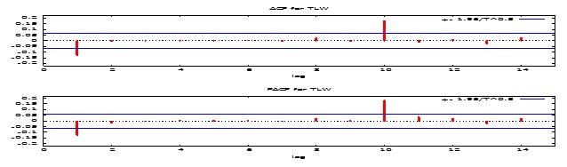 | Figure 15. ACF and PACF plot of Tullow Oil Plc Returns Series |
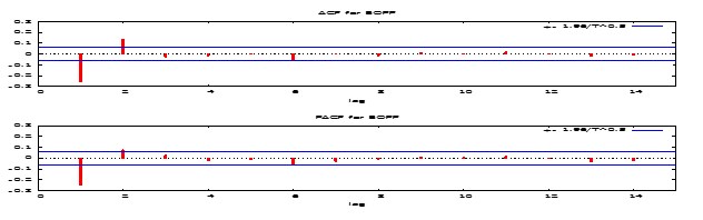 | Figure 16. ACF and PACF plot of Benso Oil Palm Plantation Returns Series |
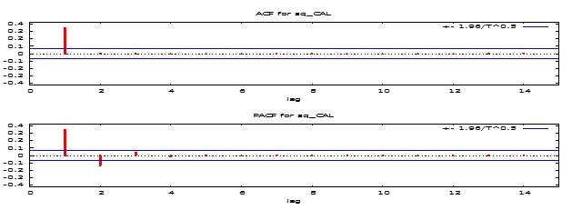 | Figure 17. ACF and PACF plot of the squared Returns Series of CAL Bank Limited |
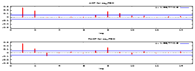 | Figure 18. ACF and PACF plot of the squared Returns Series of Produce Buying Company |
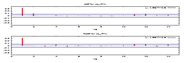 | Figure 19. ACF and PACF plot of the squared Returns Series of Fan Milk Limited |
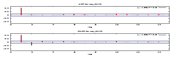 | Figure 20. ACF and PACF plot of the squared Returns Series of Clydestone (Ghana) Limited |
 | Figure 21. ACF and PACF plot of the squared Returns Series of Enterprise Group Limited |
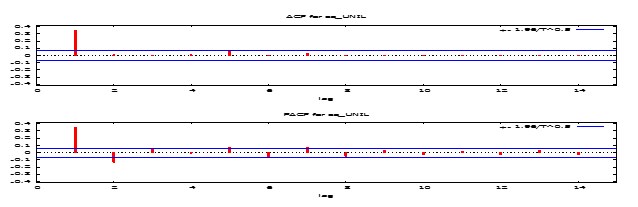 | Figure 22. ACF and PACF plot of the squared Returns Series of Uniliver Ghana Limited |
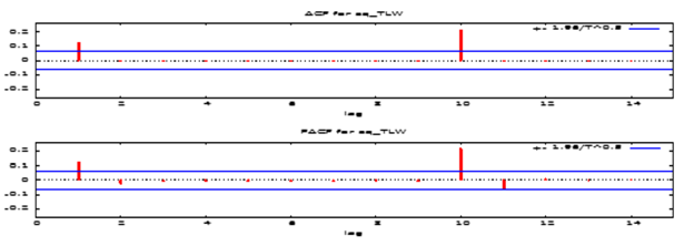 | Figure 23. ACF and PACF plot of the squared Returns Series of Tullow Oil Plc |
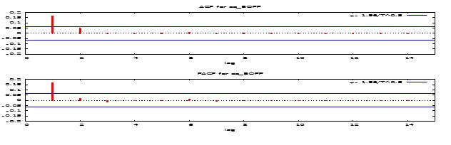 | Figure 24. ACF and PACF plot of the squared Returns Series of Benso Oil Palm Plantation |
3.2. Further Analysis
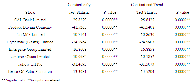
- As is reported of the ADF test in Table 2, it is evident that all the eight returns series were stationary since the p-value were significant at the 5% significance level and the null hypothesis of non-stationary was rejected.
|
|
|
|
|
|
|
 | (25) |
 | (26) |
 | (27) |
 | (28) |
 | (29) |
 | (30) |
 | (31) |
 | (32) |
|
|
4. Conclusions
- This paper modelled volatility and the risk-return relationship of some equities on the Ghana Stock Exchange using univariate GARCH models. The results revealed that, the market was good for investors since most of the equities recorded positive mean returns (gains) than negative mean returns (losses). There was high probability of making gains than losses by investors. Investing in any of the equities has its associate risk level and are highly volatile. Also, all the three models indicated that there exist a positive relationship between risk and return that is, investors were compensated for the risk assumed. The TGARCH-M (1,1) and EGARCH-M (1,1) indicated the existence of leverage effect on the market implying bad news have much effect on next period volatility than good news of the same magnitude. The TGARCH-M (1, 1) was the appropriate model since it was able to meet the model selection criterion of having the ARCH and GARCH summations mostly less than one i.e. ensuring stationairty of the model, been able to capture leverage effect and its ability in eliminate ARCH effects. It was then subjected to BIC in selecting the distributional assumption. The student-t distributional assumption was selected by the BIC. The model was then diagnosed to ascertain whether it was well specified for the returns series estimated. It was realized that, the skewness and kurtosis for the model was low for most of the returns series. Also the LB2(14) statistic was able to eliminate any further ARCH effect in the returns series. This makes the TGARCH-M (1, 1) well specified for most of the estimated returns series.