1. Introduction

Recognition of importance of infrastructure goes back to branching out of economics as a separate subject. Adam Smith was the first one who mentioned the difference of circulating capital and fixed capital, where the latter was used for “in erecting engines for drawing out the water, in making roads and wagon-ways, etc.” (Smith, 1909/2005). Similarly Karl Marx notes that ‘Among instruments that are the result of previous labor and also belong to this class, we find workshops, canals, roads, and so forth.’ (Marx, 1867/2015). However, the models of economic growth developed later in 20^th century omitted the role of infrastructure and focused only capital and labor. Thus, Harrod Domar model of 1946 focused on saving and productivity of capital, Solow-Swan Model of 1956 included labor as factor of production, Ramsey-Cass-Koopmans Model of 1965 considered that the rate of savings is endogenous and depends from consumption choice, Lucas Model of 1988 focused on human capital spillovers taking technology fixed.

Infrastructure was empirically analyzed for the first time in 1989 by Aschauer focusing on US economy. Yoshino and Nakahigashi (2000) conducted similar study for case of Japan and found statistically significant results supporting positive role of infrastructure investment.

To fill the gap of inattention to infrastructure in growth theory, we incorporate infrastructure variable as factor input into neoclassical growth model. In doing so we follow the footsteps of Mankiw, Romer and Weil (1992) who augmented the growth framework by adding human capital and conducting empirical estimation.

On the other hand, it’s very difficult to measure infrastructure and it’s subject to measurement errors, similar to that of human capital stock (Krueger and Lindahl, (2001), De la Fuente and Domenéch (2002). Considering this difficulty, many papers use infrastructure construction or launching as natural experiment and employ difference-in-difference approach to explore the nature of it’s impact. (Wang and Wu 2012, Faber 2014). In the second part of our paper we focus on case of railway connection in Uzbekistan, conduct empirical estimation using difference-in-difference approach and based on target profit pricing approach propose a framework explaining nature of infrastructure’s differential impact on outcome variables.

2. Infrastructure as an Input: Analysis of Infrastructure in Explicit Form

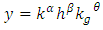
Neoclassical growth theory, upon which our modified model is based on, predicts absolute convergence for countries with the same rates of savings and population growth and access to the relatively same levels of technology. Putting it in other way, these economies will reach the same steady-state output per capita. Conditional convergence for the case of countries with different rates of saving or population growth says that steady-state outputs per capita will differ, but the growth rates will equalize (Dornbusch, 1998).

On the other hand, endogenous growth theory argues that high savings rate will lead to a high growth rate in the long run. Barro (1991; 1996) has demonstrated that while countries that invest more indeed have a tendency to grow relatively faster, the impact of higher investment on economic growth seems to have transitory nature. In other words, countries with higher investment reach steady-state with comparatively higher per capita output, but not with outperforming growth rate. Deduction which might be derived from this is as following: economies seem to converge conditionally and neoclassical growth theory addresses this question correctly. At the same time, endogenous growth theory might be of great use for analyzing the growth in advanced countries with cutting edge of technological progress.

As it were mentioned earlier Bernanke and Gürkaynak (2002) criticized the approach used by Mankiw et al. (1992) due to assumption of taking the technological progress to be evenly distributed among countries or at least having access to the same levels of technology. This assumption is difficult to be hold once you have countries which are on frontiers of technological progress and others experience huge disadvantages in this perspective; you can’t assume that firms in Denmark and Mozambique use the same level of technology for production purposes. Durlauf and Johnson (1995) using regression tree procedure derived by Breiman et al. (1984) divided Summers and Heston’s (1988) dataset into 4 groups of countries and allowed for different aggregate production functions. Surprisingly, they found positive correlation between initial level of income and long-run incomes. Dinopoulos and Thompson (1999) also support the argument that coefficients of cross-country regression with assumption of same technology and preferences should not be given much practical weight. Thus, we believe this criticism is valid and it should be accounted in estimation sample. Though it was determined by availability of data, countries in our data sample consist of only developing countries, enabling us to assume that they have access to relatively same level of technology.

To test the hypothesis of unconditional and conditional convergence controlling for public investment, we need to solve for the rate of convergence as well as derive our econometric estimation equation.

We begin with the production function in per capita terms

Growth rate in income per capita is given by

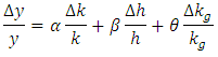Three fundamental laws of motion are:

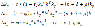Substituting this back into growth rate equation:

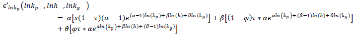
Performing Taylor approximation:

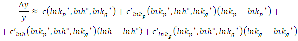From now on I calculate for and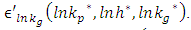

First, we have: 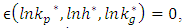because of steady state condition.

Then, solving for

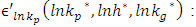
Imposing steady state:

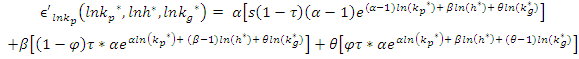Noting that:

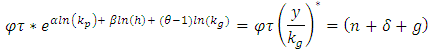We have following:

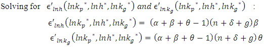Thus,

Collecting terms:

From 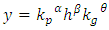it follows that:

Consequently we have:

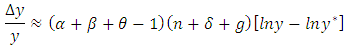Finally, the rate of convergence for our model:

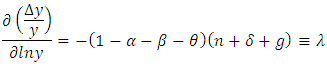Next, we need to derive our estimation equation. For this, let’s denote that:

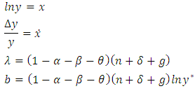Then,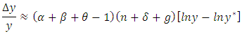

can be written as

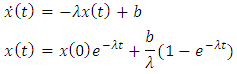Reinserting

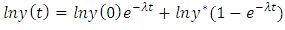In terms of growth rate:

Substituting the equation of steady-state growth for level of output:

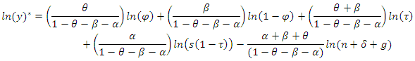We obtain estimation equation:

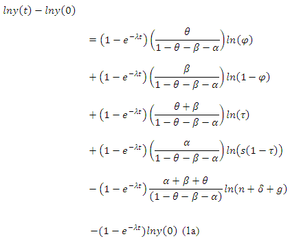
2.1. Estimation

Now applying our revised model to our sample data collected from World Bank Indicators Database, UN Population Survey Database and Barro-Lee Dataset, we test the hypothesis of unconditional and conditional convergence. For this purpose we will regress the change in the logarithm of GDP per capita for the sample period of 1991-2010 on the logarithms of GDP per capita in 1991, population growth, secondary and tertiary education as well as private and public investment using equation 1a.

First, we will test the hypothesis for absolute convergence. Next step will be using MRW’s framework to estimate the coefficients on initial level of GDP. In attempt to differentiate between secondary and tertiary education we will accomplish the regression twice, every time using different proxy variables for human capital by employing the indexes for tertiary education and secondary education from Barro Lee Dataset. After this exercises using our modified framework we estimate the parameters on private investment and public investment separately, simultaneously doing analysis of comparison between tertiary and secondary education. Finally we will test Barro (1991) and Easterly and Levine (1997) hypothesis on possibility of non-linear relationship between initial level of GDP and growth rate.

We will carry out the corresponding diagnostics for our regression, including normality test for residuals’ distribution, White’s test for detection of heteroskedasticity and Ramsey RESET test for possibilities of specification error in our equation. Finally, for the regressions with public investment the coefficient diagnostics in form of Wald test was accomplished. Table 1 and Table 2 present the estimation output and results of the corresponding diagnostics.

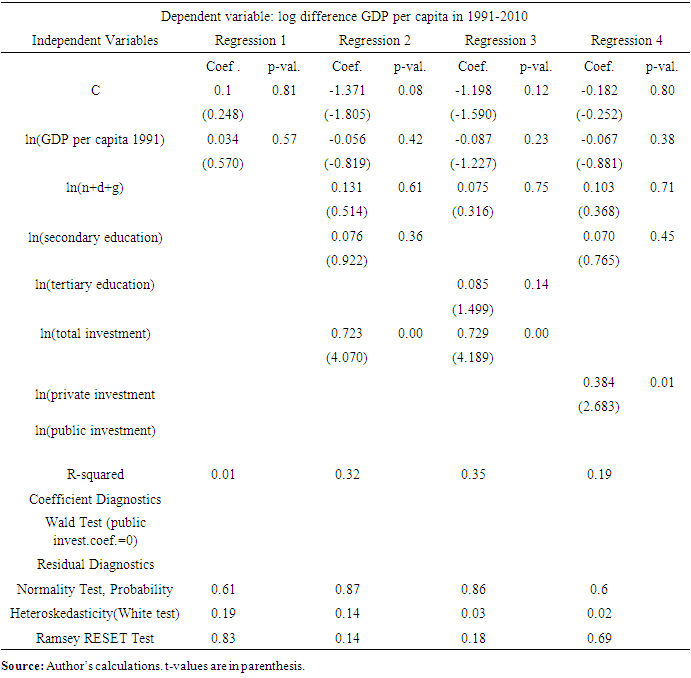Table 1. Estimation of the Augmented Model with Public Investment (part I)

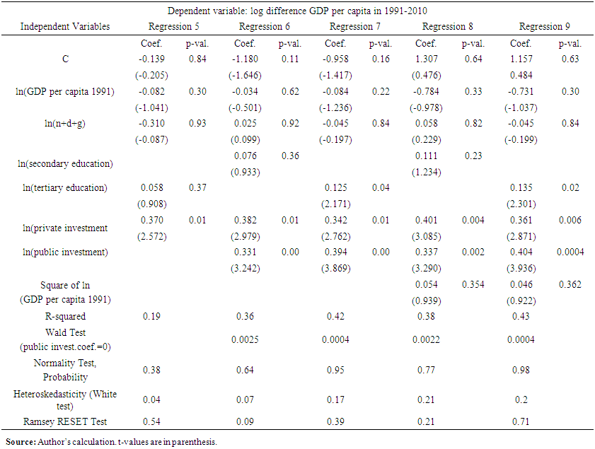Table 2. Estimation of the Augmented Model with Public Investment (part II)

2.2. Estimation Results

Our Regression 1 from the Table 1 gives the result consistent with advocators of endogenous growth theory (Romer, 1987) which constitutes the failure of incomes to converge. The same result on coefficient of initial GDP per capita was obtained by Mankiw et al. (1992). In terms of fit of the regression, R-squared is equal to 0.01.

For our Regressions 2 and 3 on Table 1 we used MRW’s framework while using Barro-Lee indexes as proxy for human capital. Consistent with the results of Mankiw et al. (1992), adding the variables for population growth, human capital and total investment makes the coefficient on initial level of GDP per capita negative, showing the tendency for convergence once the impact of above-mentioned variables are accounted for. Besides the coefficients on total investment being positive and significant, the fit for the regression improves from 0.01 to 0.35, for the case with tertiary education.

The Regressions 6 and 7 in Table 2 were carried out to observe the separate impacts of private and public investment on growth rate, simultaneously differentiating between tertiary and secondary education’s effects. However this change in right hand side of our estimation couldn’t lower the coefficient on initial level of GDP per capita in 1991, though it remained negative, supporting the convergence hypothesis.

Regressions 8 and 9 was carried out to test Barro (1991), Easterly and Levine (1997) as well as Solow’s (2003) hypothesis on non-linear relationship in growth model, in particular, between growth rate and initial level of GDP. The estimation failed to support this idea: the coefficients of squared logarithms of initial GDP per capita in 1991 found to be insignificant.

Analysis of estimation results in regard to human capital bring following conclusions: education related variables were not determined as significant for GDP growth rate until introduction of public investment in Regression 7 of Table 2. Turning to impacts of two proxy variables for human capital, the coefficient on tertiary education was always higher than that of secondary education, 0.085 vs. 0.076 and 0.125 vs. 0.076. Total investment found to be a significant determinant of growth across our estimations, with coefficients of 0.723 with secondary education and 0.729 with tertiary education as proxy variables. After separating it into private and public investment, and conducting the estimation with secondary education as variable for human capital, the coefficient on private investment was higher than that on public investment, constituting 0.382 vs. 0.331 and both being statistically significant.

However, when we used tertiary education variable instead of secondary, this decreased the size of coefficient on private investment from 0.382 to 0.342 and increased that of public investment from 0.331 to 0.394. Accomplishing the Wald test for coefficient of public investment also rejected the null hypothesis of no impact with Prob. (t-statistic) of 0.0025 for regression with secondary education and 0.0004 for regression with tertiary education. Ramsey RESET test for testing the assumption of no specification error was carried out, not being able to reject the null hypothesis with Prob(F-statistic) of 0.09 and 0.39 for estimations with secondary and tertiary education respectively.

Finally, the fit of regression in our model with separation of public investment and using tertiary education as proxy variable for human capital improved for about 30% in comparison to that obtained by using MRW framework, with R-squared being equal to 0.42 for former and 0.32 for latter.

3. Infrastructure as a Natural Experiment: Analysis of Infrastructure in Implicit Form

In this section we estimate returns from infrastructure in Uzbekistan and derive theoretical framework to explain the nature of the impact of newly provided infrastructure. We analyze impact of new railway connection on regional economic performance as observed by regional GDP and its components. Methodology we use is difference in difference approach and theoretical framework is based on target profit pricing approach.

Difference-in-difference approach allows estimating the difference between the observed, ‘actual’ outcome and alternative, ‘counter-factual’ outcome. To exercise this estimation, we need to divide the data into affected group and non-affected group on geographical basis and time basis, making the difference between pre-intervention or baseline data and post-intervention. Regression framework allows us to control for the above-mentioned covariates and obtain less biased estimate of difference in difference coefficient. Taking into account that the difference in growth rate might be occurred also due to other factors (see Rodrik (2008), Ravallion (2009), Banerjee and Duflo (2009)) we include wide range of controls into our regression framework, which takes following form:

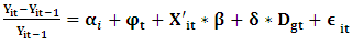(2a)

where – Regional GDP growth rate, time varying covariates(vector of observed controls), D is the binary variable indicating that observation belong to affected group after provision of the railway line, i – indexes regions, g – indexes groups of regions (1 = affected group, 0 = non-affected group), t – indexes treatment before and after (t=0 before the railway, t=1 after the railway), - sum of autonomous and time-invariant unobserved region specific rate of growth¹, year specific growth effect, error term, assumed to be independent over time.

To map out comprehensive analysis of returns we provide estimations of difference in difference under varying assumptions about timing and geography of impact. In terms of geographical impact evaluation we estimate regional effect and spillover effects, differentiating spillover effects due to adjacency and connectivity. In terms of timing impact, we examine the anticipation effect, launching effect and postponed effects from infrastructure provision.

3.1. Estimations Results

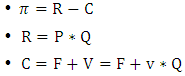
Table 3 presents estimation results for 4 versions of Equation (2a). Interaction term reported in this table, 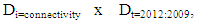focuses on comparison of trajectory for counter-factual scenario without infrastructure provision to the actual performance of the regions after launching new railway line in frame of connectivity effects (the Republic of Karakalpakstan; Samarkand, Surkhandarya and Tashkent regions) for the period of four years from 2009 to 2012, defined as ‘long-term’ in scope of our analysis. Through non-hierarchical stepwise inclusion of variables we obtain regression specification IV which is considered to be representative regression for next step of analyses². Regarding the nuisance parameters, we observe that once we control for nonlinearities proceeding from the reported in literature nature of government investments, shares of investment by population and foreign investors are identified to be significant factors of regional economic performance. These might be related to absence of agency problem and information asymmetry as compared to that of public investments. In this aspect, Afonso and Aubyn (2008) by estimating vector autoregressions for 14 European Union countries as well as Canada, Japan and the United States found that between 1960 and 2005 public investment had a contractionary effect on output in five cases, namely for GDP growth rates in Belgium, Canada, Ireland, the Netherlands and the United Kingdom, with positive public investment impulses leading to a decline in private investment, suggesting potential crowding out effects. Similar to our results, Afonso and Aubyn (2008) report that private investment impulses were always expansionary in GDP terms and effects were prevailingly higher in terms of statistical significance.

As part of sensitivity analysis we differentiate the shares of investment in total investment by sources of financing depending whether its public or private. Concerns about non-linearity and dependency of investments by state on level of government implementation (Bruckner and Tuladhar (2010)) are addressed in regressions 3 and 4 by including squared term of variable on share of public investment as well as its reciprocal. These augmentations further increases the impact of the interaction term on regional GDP growth rate pushing the size of coefficients to 2.05 and around 2.07 in regressions 3 and 4, respectively. Additionally, we identify that these point estimations become more significant in comparison to those in regression 1 and 2, with t-values in regression 3 and 4 being equal to 3.12 and 3.04, respectively.

3.2. Impact Recognition Table

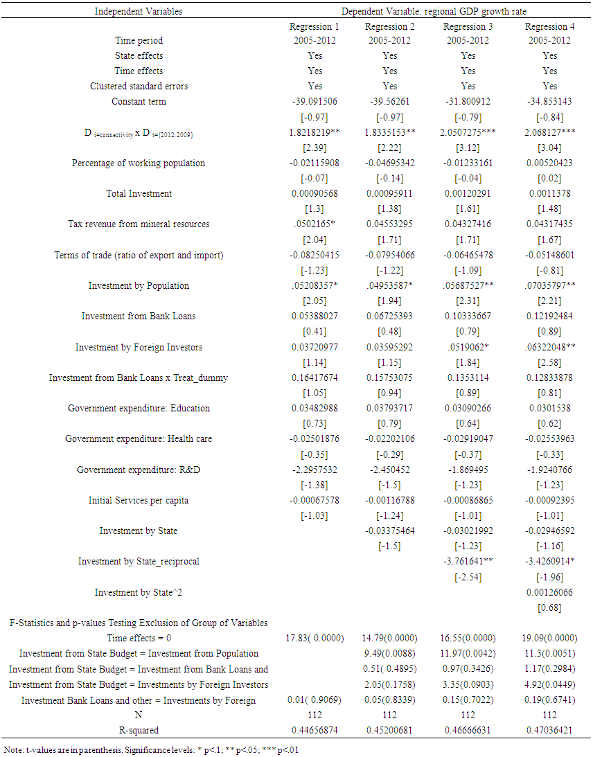
Next step, we derive impact recognition tables. To accomplish these we estimate difference in difference coefficients arising from the above-mentioned assumptions³.

Then, we report the coefficients of the interaction term, corresponding to specification adopted for regression specification IV in our Table 3 in Table 4 which contains 33 coefficients placed in accordance with chosen assumptions about timing and geographical locations, varying by dependent variable of interest.

Table 3. Difference-in-Difference Estimation Results for Regional GDP Growth Rate

Table 4. Coefficients of Difference in Difference with Outcome Variable of GDP growth rate, (growth rate percentage points)

In this way, our estimate of 2.06 with t-value of 3.04 is placed in Table 4 which reports estimation coefficients of difference in difference with variable of interest set as regional GDP growth rate. The coefficient is displayed in corresponding cell with juxtaposition of row for long-term launching effects and column for connectivity effects (see Table 4).

From Table 4 we can see that infrastructure provision’s impact after launching in the setting of spillover effects due to connectivity demonstrated positive and statistically significant effect. The regions located at the far ends of the railway system experienced 2.8, 2.5 and 2 percent higher growth rate of regional GDP in short-, mid- and long-term periods, respectively. This finding is consistent with previous empirical studies revealing positive role of distance for usage of rail as transportation mode (Wang, Ding, Liub and Xiea 2013, Jiang, Johnson and Calzada 1999, Beuthe, Jourquin, Geerts and Koul a Ndjang Ha 2000).

3.3. Theoretical Framework Based on Target Profit Pricing Approach

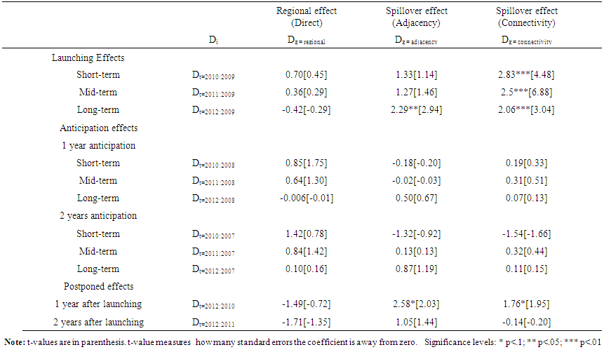
In this section we would like to explain the nature of infrastructure investment based on target profit pricing approach. We start with profit equation:

Where: P: price of goods, Q: quantity of the goods C: Total cost Profit R: Total revenue F: Total fixed cost V: Total variable cost v: Average variable cost

Taking into account that during planning period total fixed cost and average variable cost are known

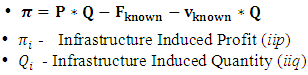(3a)

We can compute -

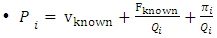Insert it back to equation 3a:

This gives:

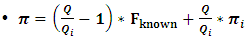(3b)

From equation 3b we can see that as long as actual sales are higher than infrastructure induced sales, actual profit will be higher than infrastructure induced profit. However, case of possible loss might be more interesting to understand. Loss is possible only if Degree of loss will depend from two factors: relative magnitudes of and relative magnitudes of

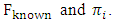To account for this we need to assume that

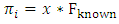Ÿ where

Replace in equation 3b gives us following:

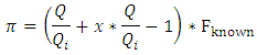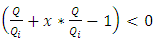
We know that total fixed cost can not be negative. Then:

When is relatively high compared to the infrastructure induced profit (when is small), a relatively small deviation of actual sales from infrastructure induced sales will result in an actual loss rather than a profit. Impact may differ depending on structure of economy of the region. Industrial (auto, machinery etc.) and Agricultural (land) sectors are associated with higher fixed costs, Services (consulting, web design etc.) are associated with lower fixed costs. As we can see from our empirical results based on case of Uzbekistan, the impact is higher on Services sector, and lower in terms of Industrial value added and Agricultural value added. Understanding these differences across regions, sectors and time is useful for understanding the nature of infrastructure impacts and formulation of corresponding policy frameworks.

4. Conclusions

In frame of this study we examined the impact of infrastructure in both explicit and implicit forms.

In explicit forms we looked at case of competitive equilibrium and derived equations for steady-state with inclusion of hard infrastructure and soft infrastructure. For this purpose we augmented neoclassical growth model and empirically estimated the direction and magnitude of infrastructure’s impact on income per capita and growth dynamics. The evidence indicates that public infrastructure investment in developing countries had positive impact on per capita income for the last two decades, though its magnitude was lower than that of private investment for about one third. In terms of impact on economic growth, public investment had greater effect than private investment once tertiary education variable from Barro-Lee dataset was used as proxy for human capital. Considered likely, education constitutes a significant determinant of economic growth, where tertiary education found to have an advantage over secondary in terms of significance and magnitude of the effect on growth rate of GDP per capita, while latter had higher impact on the levels of GDP per capita across countries.

In implicit form, we focused on case of railway connection in Uzbekistan and examined the nature of it’s impact of regional economies. Using difference in difference approach we estimated the impact of railway connection on regions of infrastructure, neighboring regions and regions located at far ends of railway system. We found that impact if is differential across regions, sectors and time. Consequently, we proposed a theoretical framework based on target profit pricing approach which could explain condition for downside deviations of economic outcomes after infrastructure provision.

ACKNOWLEDGMENTS

The authors would like to thank Georg Inderst, Sahoko Kaji, Marie Lall, Colin McKenzie, Masao Ogaki, Alfredo Pereira, Victor Pontines, and Michael Regan, as well as the participants of the Public Economics Seminar at Keio University, the AICILS conference at the University of Oxford, and the ICHE conference at Cornell University for their comments and meaningful contributions to earlier discussion of the results of the current research. Umid Abidhadjaev would also like to acknowledge the financial support provided by the Head Office of the Research Development and Sponsored Programs at Keio University under the Keio University Doctorate Student Grant-in-Aid Program.

Notes

1. Current approach requires assumption of common time path or parallel trends, accepting the autonomous rate of growth to be equal in both affected and non-affected groups.

2. This follows from property of conditional variance which states that 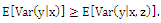(See Wooldridge, 2000). If the mean squared error (MSE) for function is defined as 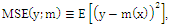then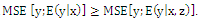

3. 4 dependent variables {GDP growth rate, Agriculture valued added, Industry value added, Services value added} x 3 geographical combinations {Connectivity, Regional, Spillover} x 11 assumptions about timing {launching effects: short-, mid-, long-term; anticipation effects: 1 year and 2 years, short-, mid-, long-term; postponed effects: 1 year and 2 year lags} x 4 specifications of regressions in total give 528 specifications of regressions.