-
Paper Information
- Next Paper
- Previous Paper
- Paper Submission
-
Journal Information
- About This Journal
- Editorial Board
- Current Issue
- Archive
- Author Guidelines
- Contact Us
American Journal of Economics
p-ISSN: 2166-4951 e-ISSN: 2166-496X
2015; 5(5): 508-512
doi:10.5923/j.economics.20150505.11
Principal Component Analysis of Nigeria Value of Major Imports
 Abstract
 Reference
 Full-Text PDF
 Full-text HTML
Usoro Anthony E.1, Moffat I. U.2
1Department of Mathematics and Statistics, Akwa Ibom State University, Mkpat Enin, Nigeria
2Department of Mathematics and Statistics, University of Uyo, Uyo, Nigeria
Correspondence to: Usoro Anthony E., Department of Mathematics and Statistics, Akwa Ibom State University, Mkpat Enin, Nigeria.
| Email: |  |
Copyright © 2015 Scientific & Academic Publishing. All Rights Reserved.
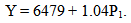
A principal component analysis of value of major imports was carried out in this research work. From the analysis, the first principal component accounted for 98.89% of the total variation amongst the observed variables. The first principal component P1 was then used as a predictor variable for subsequent analysis. The regression of the total value of major imports(Y) on the principal component (P1) yielded Y = 6479 + 1.04P1. Values obtained from the estimated model have shown reliability of the principal component approach. This paper recommends principal component analysis in a relationship between a response and multiple predictor variables to overcome the problem of multicollinearity in multiple regression analysis.
Keywords: Principal component, Eigen values, Eigen vectors
Cite this paper: Usoro Anthony E., Moffat I. U., Principal Component Analysis of Nigeria Value of Major Imports, American Journal of Economics, Vol. 5 No. 5, 2015, pp. 508-512. doi: 10.5923/j.economics.20150505.11.
Article Outline
1. Introduction
- Principal component analysis (PCA) is appropriate when you have obtained measures on a number of observed variables and wish to develop a smaller number of artificial variables (called principal components) that will account for most of the variance in the observed variables. The principal components may then be used as predictor or criterion variables in subsequent analyses. Principal component analysis is a variable reduction procedure. It is useful when someone believes that there is redundancy in some of the variables. In this case, redundancy means, some of the variables are highly correlated with one another, possibly because they are measuring the same construct. Because of this redundancy, it is possible to reduce the observed variables into a smaller number of principal components (artificial variables) that will account for most of the variance in the observed variables, Kim and Mueller [2, 3, 7, 9].Principal component analysis (PCA) is a covariance or correlation analysis between different factors. Covariance is always measured between two factors. So with three factors, covariance is measured between factors x and y, y and z, and x and z. If the there are more than three factors, the covariance values can be placed into a matrix, [4]. Principal component analysis is a mathematical procedure that uses an orthogonal transformation to convert a set of observations of possibly correlated variables into a set of values of uncorrelated variables called principal components, [5]. In principal component analysis, the number of principal components P1, P2, P3, … ,Pk extracted is always less than the number of original variables X1, X2, X3, …, Xm. The transformation is defined in such a way that the first principal component P1 account for the highest of the total variability in a multiple relationship amongst variables, and that every principal component must account for higher variability than the succeeding components, [6]. The two major terms used in analysis of principal components by Pearson (1901) are Eigenvectors and Eigenvalues. Eigenvectors can be thought of as preferential direction of a data set, or in other words, main patterns in the data. Eigenvalues can be thought of as quantitative assessment of how much a component represents the data. The higher the eigenvalues of a component, the more representative it is of the data. Eigenvalues can also be representative of the level of explained variance as a percentage of total variance in the PCA.In principal component analysis, the number of principal components is determined by the percentage of variation accounted for by the preceeding component. For instance, if the first principal component accounts for over three quarters of the total variation, subsequent principal components may not be feasible. The results of a PCA are usually discussed in terms of component scores (the transformed variable values corresponding to a particular data point) and loadings (the weight by which each standardized original variable should be multiplied to get the component score), [8]. Principal component analysis has been one of the most valuable results from applied linear algebra. It is used abundantly in all forms of analysis from neuroscience to computer graphics, because it is a simple non-parametric method of extracting relevant information from confusing data sets. It provides a road map to the reduction of a complex data set to a lower dimension in order to reveal the sometimes hidden simplified structure that often underlie it, [1]. [10] described principal component analysis as an analysis whose purpose is to introduce new variates (called principal components), which are linear combination of the original variables X’s in a multiple relationship amongst the variables of interest, such that the principal components obtained are orthogonal. One of the reasons of adopting principal component method is to solve the problem of multicollinearity in a multiple regression model. [10] carried principal component analysis, using correlation matrix and extracted two principal components from the original five explanatory variables in a multiple relationship amongst the variables of interest. [4] used covariance matrix for the analysis of the principal component. In this paper, we intend to analysis Nigeria’s value of major imports through principal component method.
2. Statistical Method
- This Section contains the procedure involve in the calculation of the eigenvalues in the principal component analysis.
2.1. Source of Data
- The source of data for this research work is from page 198 of Central Bank of Nigeria Statistical Bulletin Volume 21, December, 2010. Particularly, Value of major imports is our study interest. The total value of major imports is aggregation of the following components: Food & Live Animal Beverages & Tobacco, Crude Materials Inedible, Mineral Fuels, Animal and Vegetable, Oil & Fat, Chemicals, manufactured goods, Machinery & Transport Equipment, Miscellaneous Manufactured Goods and Miscellaneous Transactions. In this paper, we have conveniently removed the last two components, since their details are not reflected in the bulletin.
2.2. Description of Variables
- The variables used for the analysis are defined as follows:Total Value of Major Imports (Y)Food & Live Animal (X1)Beverages & Tobacco (X2)Crude Materials Inedible (X3) Mineral Fuels (X4)Animal and Vegetable (X5)Oil & Fat (X6)Chemicals (X7) Manufactured Goods, Machinery & Transport Equipment (X8)
2.3. Correlation Matrix
- The correlation matrix for each pair of variables is given below:
2.4. Principal Loadings for the Principal Component
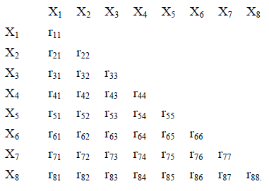
- [10] expressed loadings for the first, second, third ,…, kth principal components as:L1j, L2j, L3j, …, Lkj (j = 1, 2, 3, …, 8).L1j = r.j/√r.., j = 1, 2, 3, …, 8.r.j are the column sums from the correlation coefficient for a particular principal component. r.. is the sum of all the correlation coefficients for a particular principal component.
2.5. Eigenvectors for the Principal Component
- The percentage of variation accounted for by “k” number of principal components is expressed by Eigenvectors, whose values are obtained from the principal loadings. The eigenvectors are λi (i = 1, 2, …, k). λ1, λ2, λ3, …, λk are the eigen vectors for the ‘k’ number of principal components. Therefore, the percentage of variation accounted for by a principal component, say P1 is P1% = λ1/k percent. K is the number of X’s in original data. This expresses the proportion of the total variation accounted for by each principal component, and also gives an idea as to whether subsequent principal components are significant or negligible in the analysis.
3. Estimation and Analysis
- Here, we apply the aforementioned statistical procedure for the extraction of the principal loadings and components.
3.1. Matrix of Correlation Coefficients
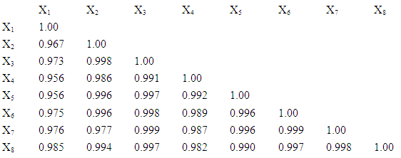 The column sums of the correlation coefficients are r.1 = 7.788, r.2 = 7.914, r.3 = 7.953, r.4 = 7.883, r.5 = 7.923, r.6 = 7.95, r.7 = 7.932, r.8, = 7.943. The sum of the column totals of the correlation coefficients is r.. = 63.286. √r.. = √63.286 = 7.955.
3.2. Loadings for the First Principal Component and Its Percentage of Variation
- The loadings for the first principal component are estimated as follows:l1j = r.j/√r..l11 = 0.9790, l12 = 0.9948, l13 = 0.9917, l14 = 0.9909, l15 = 0.9960, l16 = 0.9994,l17 = 0.9971, l18= 0.9985. The principal component is P1 = L11X1 + L12X2 + L13X3 + L14X4 + L15X5 + L16X6 L17X7 + L18X8. From the estimated loadings, the principal component model is obtained as,
 | (1) |
3.3. Regression of total Value of Import on the Principal Component
- The final analysis in this paper is the regression of the total value of import on the principal component. As mentioned in the introductory part of this paper, P1 is going to act as a predictor variable in a simple regression analysis. This is an alternative approach to multiple regression analysis of the total value of import on the X’s. Therefore, the regression of Y on P1 yields the following model,
 | (2) |
|
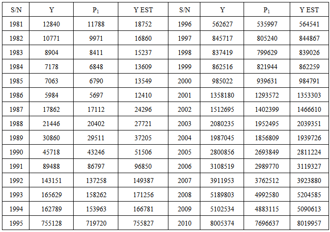
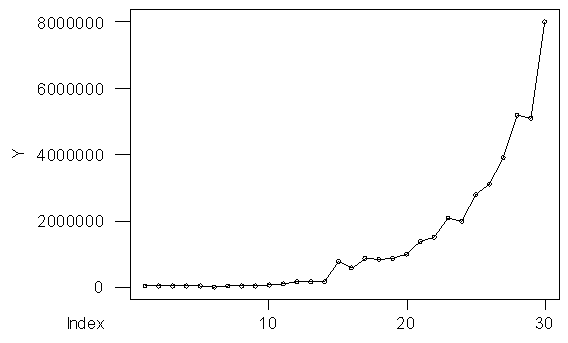 | Figure 1. Gtaph of original values |
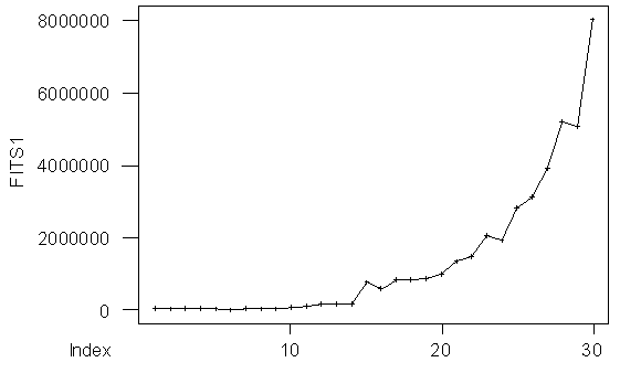 | Figure 2. Gtaph of the estimates |
4. Conclusions
- Principal component analysis is a powerful tool for reducing a number of observed variables into a smaller number of artificial variables that account for most of the variance in a given data set. It is an explanatory tool to uncover unknown trends in a given set of data. The number of principal components extracted from the observed variables is determined by the percentage of total variation accounted for by the first principal component. The analysis carried out in this paper has revealed that the first principal component P1 has accounted for almost the total variation amongst the observed variables. This further explains the fact that subsequent principal components are insignificant and negligible. Principal component method is useful, especially, when the explanatory variables are strongly correlated. Strong correlation amongst pairs of variables is synonymous with multicollinearity. So with principal component analysis, problem of multicollinearity in a multiple relationship between response and predictor variables is addressed.