Hilal Yildiz 1, Seda Atasaygin 2
1Faculty of Economics and Administrative Sciences, University of Kocaeli, Umuttepe Campus, Kocaeli Turkey
2Regional Sales Manager of Marmara, Finansbank, Kocaeli, Turkey
Correspondence to: Hilal Yildiz , Faculty of Economics and Administrative Sciences, University of Kocaeli, Umuttepe Campus, Kocaeli Turkey.
| Email: |  |
Copyright © 2015 Scientific & Academic Publishing. All Rights Reserved.
Abstract
The relationship between financial deepening and economic growth has been debated extensively in the literature. The causal relationship of the finance-growth nexus has important policy implications for the economy. The study examines the relationship between financial deepening and economic growth in the Turkish economy for the period from 1984:01-2014:12. The industry production index is used as representative of economic growth. The variables of the stock index of Istanbul, bonds and stocks are used as financial development indicators. We conclude that there is a cointegration relation among variables. According to our results, the demand-pulling hypothesis is valid for the Turkish economy. We find that there is evidence that the growth of the economy in recent years has substituted for financial development. The work is divided into five sections. Section one is the introduction, section two deals with the theoretical literature review of the relationship between economic growth and financial development, and section three discusses the empirical literature. Section four analyzes the data and discusses the findings under the empirical results while section five discusses the conclusion.
Keywords:
Growth, Financial deepening, Causality, Cointegration, Turkey
Cite this paper: Hilal Yildiz , Seda Atasaygin , Financial Deepening and Economic Growth: The Turkish Experience, American Journal of Economics, Vol. 5 No. 5, 2015, pp. 477-483. doi: 10.5923/j.economics.20150505.06.
1. Introduction
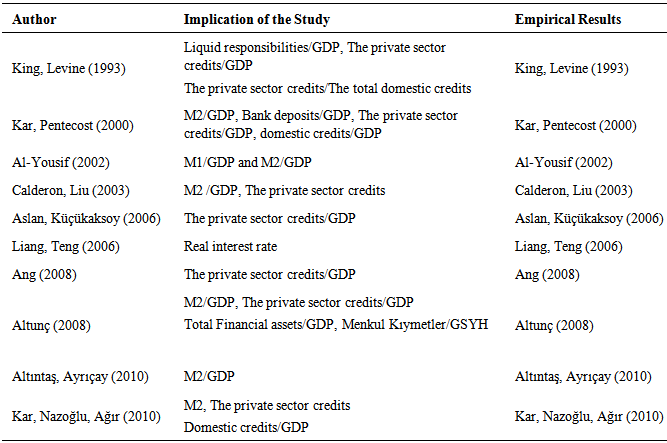
The increase of financial assets in the financial system and broadly using them is called “financial development” (Erim, 2005). Also, it is identified as the changing of the financial system in terms of structure and size. It is important to note that if the increase in the supply of financial assets is small, it means that financial deepening in the economy is most likely to be shallow; but if the ratio is big, it means that financial deepening is likely to be high. Developed economies are characterized by high financial deepening, meaning that the financial sector in such countries has had significant growth and improvement, which has, in turn, led to the growth and development of the entire economy. Financial deepening is a term used often by economic development experts. It refers to the increased provision of financial services with a wider choice of services geared to all levels of society. It also refers to the macro effects of financial deepening on the larger economy. It means that the size of financial assets increases more than the size of non financial assets in the economy (Shaw, 1973). There are many indicators for estimates of financial development. There is no unique parameter in the measure of financial development. There are five indicators such as the indicators of quantity, structure, the price of finance, cost of change and product range (Darıcı, 2009). The main indicators of financial development are summarized at Table 1.Table 1. The Main Indicators of Financial Deepening
 |
| |
|
2. The Relationship between Economic Growth and Financial Development
The relationship between financial development and economic growth has been debated extensively in the literature. The causal relationship of the finance-growth nexus has important policy implications for the economy. Walter Bagehot made the first attempt at evaluating the relationship between financial and economic development in 1873 (Becsi and Wang, 1997:50). The original debate on the relationship between financial development and economic growth can be traced to Schumpeter, who argues that economic growth is affected by the financial system. The important question is that in the relationship between financial development and economic growth, which one leads in the dynamic process of economic development?Most of the studies have focused on the effect of the financial system on economic growth in the literature. The direction of the relationship between financial deepening and economic growth is the crucial guestion. According the general approach, the effect of the financial system on economic growth is passive. But the modern approach claims that the effect of the financial system is active on economic growth (Hermes and Lensink, 1997:7). There are different wiews in the literature. The first hypothesis is that economic growth causes financial development. The other main hypothesis argues that economic growth is caused by the financial system.
2.1. The Demand-Pulling Hypothesis
It was introduced by Robinson in 1952. In this hypothesis, the main thinking is that “the financial development follows economic growth”. It argues for a reverse causal ordering from real economic growth to financial development that is a consequence of economic growth, as economic growth increases demand for financial instruments. The growth of the real economy causes the increase of labor productivity and technological development. As a result of expansion of the real economy, the economy needs more financial intermediaries. In that concept, the financial system plays a passive role in the economic growth process (Calderon and Liu, 2003:326).
2.2. The Supply Leading Hypothesis
This hypothesis assumes that the direction of causation runs from financial development to economic development, and emphasizes the role played by financial liberalization in increasing savings and investment. In this concept, economic growth can be the combined role of investment and financial deepening. The effective financial market contributes to invesment and economic growth (Rioja and Valev, 2004:127). The effect of financial development on economic growth occurs in two ways:- The development of the financial system leads to the increase of efficiency of capital flows. - It leads to increase of saving and invesment (Gregorro and Guidotti, 1995:5). The new tools that arose from the financial system lead to increased demand in the real sector. The determinators of the real sector are caused by financial activities. The direction of the relationship between economic growth and financial deepening is from the financial system to the real economy. The productivity and value added are created by saving, invesment, the minimizing of risks and decreasing of costs. The financial development leads to the accomodation of saving. The increase of saving creates new invesment and increasing invesment causes economic growth.
3. The Review of Related Literature
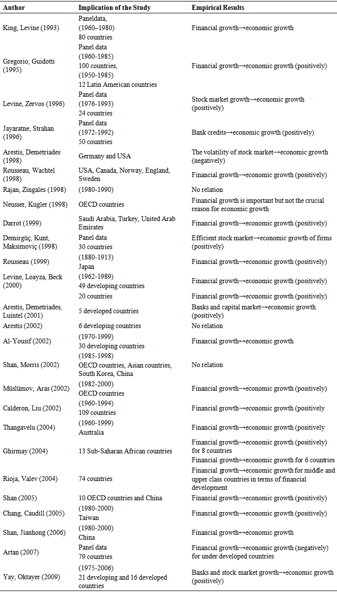
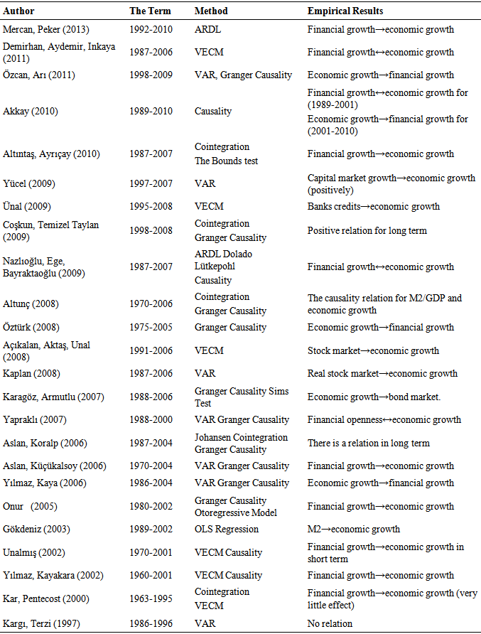
The literature related to the relationship between financial deepening and economic growth is summarized at Table 2 and Turkey’s empirical experiences are summarized at Table 3. Most of them indicate that there is positive relation between variables but the direction of relation is mixed. Some of them found that the demand-pulling hypothesis is valid, most of them reached an opposite hypothesis. Table 2. Literature Survey
 |
| |
|
Table 3. Literature Survey of the Turkish Experience
 |
| |
|
4. Empirical Analysis
In this study, Engle-Granger Model was used to estimate the short-run and long-run relationship between financial deepening and economic growth in Turkey. Firstly, we discussed the data set and details of the Engle-Granger model (EGM).
4.1. Data
In our empirical analysis, we used monthly data set of 1989:01-2014:12. Industry production index (IPI) was used as a proxy for economic growth. As financial deepening indicators, we used bonds (B), stock index of Istanbul (SI), and stocks (S). The data were obtained from the Central Bank of the Turkish Republic. In view of the foregoing, the functional relationship between financial development and economic growth that incorporates various proxies of financial sector development (explanatory variables) for estimation purpose is specified.
4.2. Methodological Framework
Before analyzing the relationship between economic growth and financial deepening, both dependent and independent variables are subjected to some statistical tests such as stationary test. Augmented Dickey-Fuller (ADF) (Dickey, Fuller, 1979) is used to find out the stationary of any time series. This is necessary in order to ensure that the parameters are estimated using stationary time series. The essence of the ADF tests is the null hypothesis of nonstationarity. To reject this, the ADF statistics must be more negative than the critical values of Dickey-Fuller table. Why is it important to use the stationary variables in the econometrics analysis? The reason is that standard regression analysis fails when dealing with non-stationary variables, leading to spurious regressions. For example, suppose we regress two independent random walks (nonstationary) against each other, and test for a linear relationship? A large percentage of the time, we'll find high R-squared values and low p-values when using standard OLS statistics. In fact, there's absolutely no relationship between the two random walks (Enders, 2004). On the other hand, if the variables are not stationary at level (I(0)), we have to take their difference form (I(1)). Using the difference form of the variables leads to lack of long term knowledge. At that point, Granger suggests the cointegration form as a technique to observe the relationship between integrated variables. If two or more series are individually integrated but some linear combination of them has a lower order of integration, then the series are said to be cointegrated. A common example is where the individual series are first-order integrated (I(1)) but some (cointegrating) vector of coefficients exists to form a stationary linear combination of them (Charemza, Deadman 1992). To avoid this, Engle and Granger (1987) provided a remedy. The EGM, originally suggested by Engle and Granger (1987), has received a great deal of attention in time series analysis. It gives the long-run equilibrium relationship between variables, which can be modeled by the regression involving the levels of the variables. Firstly, the regression is estimated by the OLS.  | (1) |
Where both Y and X are nonstationary variables and integrated of order one ( i. e. Xt ∼ I(1) and Yt∼I(1)). In order for Yt and Xt to be cointegrated, the necessary condition is that the estimated residuals from the equation should be stationary (i. e. ut∼ I(0)). ut is called an error correction term if it is found by stationary. Secondly, conditional on finding cointegration between Yt and Xt, the estimate of β from the first step long-run regression (1) may then be imposed on the following short-run model with the remaining parameters being consistently estimated by the OLS. In other words, we retrieve the estimate of β from Eq. (1), and insert it in place of β in the error-correction term (Ct-βYt) in the following short-run equation: | (2) |
Where Δ represents first-differences and εt is the error term. Alternatively, in practice, since Ct-βYt = ut, one can substitute the estimated residuals from Eq. (1) in place of the error-correction term, as the two will be identical. Note that the estimated coefficient α2 in the short-run Eq. (2) should have a negative sign and be statistically significant. Note also that, to avoid an explosive process, the coefficient should take a value between -1 and 0. According to the GRT, negative and statistically significant α2 is a necessary condition for the variables in hand to be cointegrated. In practice, this is regarded as convincing evidence and confirmation for the existence of cointegration found in the first step. It is also important to note that, in the second step of the EGM, there is no danger of estimating a spurious regression because of the stationarity of the variables ensured. Combinations of the two steps then provide a model incorporating both the static long-run and the dynamic short-run components (Yıldız, 2013).
4.3. Empirical Results
In this section, the result of the augmented unit root test of the series, cointegration test among variables and VECM causality test are presented in tables and analyzed as follows. Table 4 shows that the null hypothesis of unit root is not rejected because the test statistic is not more than the critical values at level. The absolute values of the test statistic of the series are greater than the critical (absolute) values of the series at 5 percent level of significance at first difference. Thus, the series is stationary at the first difference and at 5% level. Table 4. The Results of ADF Test
 |
| |
|
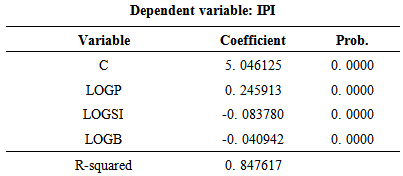
Table 4 presents the results of ADF statistics for the levels and first differences of the monthly time series data for the period, 1989:01-2014:12. The asterisk (*) denotes rejection of the unit root hypothesis at the 5% level. As follows, Tables 5, 6, 7 and 8 show, respectively, error-correction results of variables at level, the results of VECM, the diagnostic test of VECM and wald test results of VECM for which the dependent variable is the stock index.Table 5. The Results of Error-Correction Regression at Level
 |
| |
|
Table 6. The Results of VECM
 |
| |
|
We need to observe the cointegration relationship, for which the error correction term must be stationary at level. Firstly, we regressed the variables at level in which the dependent variable is IPI. Then, we checked the stationary of the error term of the regression at Engle-Yoo table. According to the critical values of the table (3. 47), the error correction term is stationary at 10% (Engle-Yoo, 1987, Table 2:157). Thus, we can observe the cointegration relation among variables.According to the VECM results at Table 6, the error correction mechanism (ECM) (-4. 3642) works only for the SI as a dependent variable. The error correction term is statistically significant at 5% and has a negative sign. This means that the error correction mechanism works. ECM is the error correction component of the model and measures the speed at which prior deviations from equilibrium are corrected. Table 7 gives the results of wald test for VECM. According to the results, in the regression in which the dependent variable is SI, there exist the short and long term relation among variables both of joint test and wald. All of the variables (IPI, S and B) have impact on SI which is the dependent variable. The diagnostic tests indicate that there is no econometrics problem such as autocorrelation and heteroscedasticity in the estimation result. Table 7. The Results of Wald Test in VECM
 |
| |
|
Our Turkish experience supports Robinson’s view. The financial market is followed by the real market. The impact of economic growth on the financial market has been demonstrated in the same way as ours by Onur (2005), Kar and Pentecos (2002).
5. Conclusions
The objective of this study was to analyze the relationship between economic growth and financial deepening for Turkey. To establish the direction of causality among financial development and economic growth, the cointegration was employed using three alternative financial proxies, the stock index of Istanbul, bonds and stocks. Empirical evidence from the error correction testing approach to cointegration suggested that there existed only one long-run relationship between the alternative financial development proxies and economic growth. In order to observe the validity of demand-pulling or the supply-leading hypotheses in the case of Turkey, VECM causality tests revealed that changes in the economic growth, through the error-correction term, resulted in changes in financial deepening in the long-run, via the stock index of Istanbul.
References
| [1] | Altıntaş H, Ayrıçay Y. (2010). “Türkiye’de Finansal Gelişme ve Ekonomik Büyüme İlişkisinin Sınır Testi Yaklaşımıyla Analizi” Anadolu Üniversitesi Sosyal Bilimler Dergisi, 10(2): 71-98. |
| [2] | Ang, J.B (2008) “What Are The Mechanisms Linking Financial Development and Economic Growth in Malaysia?”. Ecenomic Modelling, (25), 38-53. |
| [3] | Aslan Özgür, İsmail Küçükaksoy (2006). “Finansal Gelişme ve Ekonomik Büyüme İlişkisi: Türkiye Ekonomisi Üzerine Ekonometrik Bir Uygulama”. İstanbul Üniversitesi İktisat Fakültesi Ekonometri ve İstatistik Dergisi, (4):25-38 |
| [4] | Al-Yousif, Yousif Khalifa (2002). “Financial Development and Economic Growth: Another Look At the Evidence From Developing Countries”. Review of Financial Economics, (11):131-150. |
| [5] | Besci, Z, Wang P (1997). “Financial Development and Growth”. Federal Reserve Bank of Atlanta Economic Review, 82(4):46-62. |
| [6] | Calderon, S, Lui, L (2003). “The Direction of Causality between Financial Development and Economic Growth”. Journal of Development Economics, 72(1):321-334. |
| [7] | Chaaremza, Wojciech W, Derek F. Deadman (1993). Econometric Practice. Vermont. |
| [8] | Dickey, D.A. and W. A. Fuller (1979). Distribution of estimators for autoregressive time series with a unit root. Journal of the American Statistical Association 74, 366. |
| [9] | Dickey, D. A., and W. A. Fuller (1981). Likelihood ratio statistics for autoregressive time series with a unit root. Econometrica 49 (4): 1057–72. |
| [10] | Enders, W (2004). Applied Econometric Time Series. USA. |
| [11] | Engle, R.F; C. W. J. Granger (1987). Co-Integration and Error Correction: Representation, Estimation, and Testing. Econometrica, Vol. 55, No. 2 |
| [12] | Gujurati, Domadar (1999). Temel Ekonometri. Literatür Yayınları. |
| [13] | Hermes Niels, Robert Lensing (1996). Financial Development and Economic Growth. New York and London: Routhledge. |
| [14] | Kar, Muhsin, Şaban Nazlıoğlu, Hüseyin Ağır (2010). “Financial Development and Economic Growth Nexus İn the Mena Countries: Bootstrap Panel Granger Casuality Analysis”. Economic Modelling, (28):685-693. |
| [15] | Kar, Muhsin, Eric J Pentecost (2000). “Financial Development and Economic Growth in Turkey: Further Evidence On The Causality İssue”. Loughborough Univercity, 1-20. |
| [16] | Levine, R, S. Zerous (1996). “Stock Market Development and Long-Run Growth”. World Bank, Working Paper, 1582. |
| [17] | Levine, Ross (2004). “Finance and Growth: Theory and Evidence”. Nber Working Paper Series, (10),766. |
| [18] | Levine, Ross (1997). “Financial Development and Economic Growth: Vievs and Agenda”. Journal of Economic Literature, 35(2),695. |
| [19] | Levine, Ross (2001). “Bank Based or Market Based Financial System: Which İs Better?”. Carslon School of Management Univercity of Minnesota. |
| [20] | Rioja, F, N. Valeu (2004). “Finance and The Sources of Growth at Various Stages of Economic Development”. Economic Ingury, 42:127-140. |
| [21] | Shaw, E (1973). “Financial Depening İn Economic Development”. Oxford Univercity Press, London. |
| [22] | Yıldız, Hilal (2013). Zaman Serileri Analizi. Bursa: Ekin Yayıncılık. |
| [23] | Demir, Osman (2004). “İçsel Büyüme Kapsamında Devletin Değişken Rolü” http://www.bilgiyonetimi.org |
| [24] | Yumuşak, İbrahim Güran, Yusuf Tuna (2004). “Kalkınmışlık Göstergesi Olarak Beşeri Kalkınma İndeksi ve Türkiye Üzerine Bir Değerlendirme”. http://www.bilgiyonetimi.org |


 Abstract
 Reference
 Full-Text PDF
 Full-text HTML