1. Introduction

Failure of the UR and the bog of the DDA in reaching a consensus in contentious sectors and meeting the interests of developing countries (especially the least developed among them) particularly in agriculture, multilaterally, has compelled groups of countries to resort to Regional Trade Agreements (RTAs) to hasten and consolidate their trade gains (Head & Ries, 2004; Kessie, 2004; OECD 1997). The proliferations of these new RTAs exude an increasing level of sophistication, both in terms of scope and configuration than ever experienced before. Also, agriculture plays an important and twin part in them, especially, the South-South (S-S) cooperation and integration blocs than seen before. Agriculture is significant for exports and essential for intra-bloc trading in merchandise. S-S intra-and-inter bloc markets provide a safer scope for maximizing gains from trading in food and agriculture raw materials than otherwise. This is attributed to improved market access policies and the implementation of intra-bloc production support much faster and readily, than it would be at the international level.

Of the sub-components of the agriculture sector, food item trade provides the RTAs’ member countries with the best attempt for faster development and elimination of poverty, since it involves stages in value addition that enhances more export gains compared to agricultural raw materials exports. In contrast, processed merchandise from S-S countries face higher tariffs and other restrictions related to quality and standards that bar them from enjoying these gains, when they export to the lucrative markets in the North. This inadvertently compromises the gains therein since developing countries production and trading structure is still incompetent to much up to such restrictions. However, there is a scare at the scope and speed of such trade liberalization of typically the food sector in comparison to the liberalization of other sectors such as agricultural raw materials, fuels, ores and metals, and manufactures on the other side. Normally, trade liberalization measures in the food or even agricultural sectors inhibit efforts to increase intra-bloc trade and undermine food security rather than uplift efforts to reduce poverty as Vylder (2007) argues.

Such conclusions have bred empirical interest as to whether the efforts of the East African Community (EAC) are paying off, more so, the bloc’s ambitions in securing the gains are commendable. Among the S-S blocs, EAC member states have exuded the fastest and most significant liberalization measures, and incurred huge sunk costs in reconfiguring the bloc from an FTA to now a common market in less than 10 years. It is hoped to become a political federation (the highest and most complex level of integration) by 2015. However, a survey of the literature on RTAs hardly reveals any empirical literature on EAC to solve such empirical interest and it has neglected trade in food item.

Much as the massive changes and commitments in EAC food or agrifood sector was and is presumed to impact significantly on agrifood trade in the region, the extent to which these policies have impacted on agrifood trade is however not known or even documented. This could possibly be due to limited and inadequate empirical studies guiding the evolution of the EAC and the process of formulating its policies. The limited studies available on this are tainted with strong statements, theory and causal empiricism rather than robust empirical studies and theories. Studies like Wanjiru, (2006); Gregory, (1981); Kirkpatrick & Wantabe (2005); Ochwada, (2004) written on EAC, are too general to answer the pertinent issues evolving in the bloc, and as such, are devoid of their explicit policy outcomes and intention to guide sectoral or specific policy needs of the bloc. Studies on RTAs, though exclusive of EAC dynamics have also not paid attention to the effects or impacts of these trading blocs on agrifood trade, a core area that this study tackles. The methodologies and econometric processes adopted by these studies have even most times been spurious. The data was not as disaggregated as the one this study utilized.

In this regard, this study examined the postulation that trade liberalization (regional integration) policies of LDCs normally undermine their presumed impact. It was based on the experience of EAC trade agreement. It adopted the extended gravity model, to analyze the impact of this regional integration on food item. The model includes 168 countries and is estimated with panel data over the period 1988 – 2009. A Poisson estimation method that took into account unobserved trade data characteristics of the bilateral trade relations was estimated.

2. Theoretical and Empirical Evidence

2.1. Theoretical Underpinnings

There are three broad categories of theories that have emanated in the literature to explain and measure trade between countries, including; the canonical or classical, the neo-classical and the “new trade” theories. By design, they analyze trade in general merchandise, though do not explicitly analyze trade in agrifood or food items. However, since the modified ones explicitly make the linkages (through dummies or incorporating the agrifood products as endogenous flows) between RTAs and effects on agrifood trade, they may be construed to study food item trade.

The classical or traditional trade theories governed trade in the world from the 16^th to 18^th centuries was the formative trade theories. They assumed that countries are different, and this difference explains the pattern and gains from trade in the different products. During this time, there were three theories explaining trade starting with mercantilism in 1500 – 1750, to Adam Smith’s Absolute Advantage theory and David Ricardo’s Comparative advantage. Mercantilism emphasized that a country keeps a positive trade balance to safeguard it during war and guarantee prosperity. To maximize a positive trade balance, exports were promoted and imports discouraged. In this model, since a country gained at the expense of another, this trade was not considered mutually beneficial. Mercantilist trade policy was viewed as ‘zero-sum’ game and led to resentments, revolts and progressive wars that made such a practice or idea untenable. Over time, mercantilism lost its appeal, and was readily replaced by yet another theory - the theory of absolute advantage that emphasized ‘win-win’ outcomes in trade. The idea behind this theory was that, a trade regime could be changed by producing only commodities of absolute advantage and exchange (trade) the surplus of this process with a trading partner who specializes in producing commodities that are domestically expensive to produce, hence benefiting also consumers and gains from trade. Intuitive as it was, the theory failed to explain the pattern and gains from trade when a country is disadvantage in all ranges of products. More to this, it only explained a small part of world trade and it is seen as a special case of the more general theory of trade based on comparative advantage which refined the absolute advantage theory. David Ricardo introduced the theory of comparative advantage theory, that had models that differed in structure from absolute modules but aimed at explaining the pattern of and gains from trade (inter industry). Customary, they were based on the law of comparative advantage (Either 1983 & Salvatore 2004) which provided a solution to the impasse created by the absolute advantage theory. These models specify that mutually beneficial trade can still occur between two nations even if a country is less efficient in the production of two commodities. This is enabled when each nation specializes and trades (or exports) the commodity in which it has less comparative disadvantage and import the commodity of more comparative disadvantage. However, in time, major flaws were also cited in these models: First, the models imply complete specialization in production, which is not tenable; secondly, there is an assumption of a single factor of production. Countries produce major production simultaneously, and further, the models fail to incorporate income distributions issues and there is doubt that assumption of technological differences can posit in the long run across countries.

The failings in the classical trade theories gave rise to a new group of theories known as the neo-classical or standard trade theories. The standard trade models assume that there is a variant of factors of production, an issue not considered in the classical trade theories. And that the difference in resources can drive the trade patterns and this affects the distribution of resources (Krugman & Obstfeld, 2009). The two major models that fall in this category are the Heckscher - Ohlin and Ricardo-Viner models. The Heckscher - Ohlin model assumes that factor abundance will determine the pattern of and gains from trade in those products it is endowed with. This is because they will have a comparative advantage in producing those products. However, this could only hold if the economy’s major sectors have wages above the subsistence level (Vylder 2007). While the Ricardo-Viner model emphasizes the fact that trade patterns will be reflected by factor abundance across countries when production technologies are identical across countries. Intuitive as these models are, they still failed to estimate trade fully since issues that affect political debate (like migration, growth, transit costs, and network effects) today were still exogenous to these models, hence a rise of a totally new group of theories after the Second World War.

The 1970s and 1980s saw an emergence of a new range of trade models broadly labeled New Trade Theories (NTT). They too considered increasing returns to scale that enable firms, industries or sectors to build a huge competitive world market base. The other presumptions related to the emphasis of NTT on networks (mainly their effect), and monopolistically competitive industries producing differentiated products. These monopolistically competitive industries engaged in intra-industry-trade (exchange of same product but of different variety) (Krugman & Obstfeld, 2009). At their evolution, the models of the NTT lacked sufficient dataset to test them empirically. Further, besides being too technical, empirically produced mixed results and their reliability produced mix results, the statistical judgments from them were hard to fathom. More to this, the time-scales required and the particular nature of production in each 'monopolizable' sector was subjective to the researchers. Prior to the evolution of the NTT, there was increased interest that stemmed to analyze the outcome of RTAs or EIs specifically. Traditionally, this economic analysis evaluated the desirability of regional integration arrangements according to their trade diversion and trade creation effects (Shams 2003). Viner’s seminal work on trade creation and diversion effects in 1950, noted that trade creation occurs when imports are substituted for domestic products as a result of tariff reductions that reduce the price of member imports below that of home-produced goods. While trade diversion transpires with a shift in imports from an efficient non-member exporter to a more expensive producer from the country’s RTAs partners due to preferential tariff treatment. Trade diversion, in Viner’s view, did not necessarily mean a decline in trade, but rather a shift in trade away from the least cost suppliers. Contemporary writers simply state that, trade creation occurs if partner country production displaces higher cost domestic production. And trade diversion implies that partner country production displaces lower cost imports from third countries. Trade diversion is said to increases intra-bloc trade at the expense of trade with third countries, while trade creation does not have this negative effect. Therefore a regional trade arrangement is only desirable if trade creation outweighs trade diversion (Shams 2002).

Another model that evolved during this same period is the Gravity model. And it has been widely used in analyzing trading patterns better than many of the theoretical models on trade. The gravity model, tries to incorporate a broad range of covariates lacking in theoretical models discussed above. Furthermore, the gravity analysis and model has gained supremacy due to the fact that it has a predictable role as a tool used in estimating effects of a variety of phenomena in social sciences. In economics and especially international trade, it is a successful modeling approach for various reasons; the results from it have high explanatory power of between 0.65 and 0.95 and are sensible (especially on distance and output), economically and statistically significant. Also, there is easy access to bilateral trade data, and the model explains most of the variations in international trade. Estimation standards and benchmarks of the gravity model have been clearly established. The next section reviews the build - up of the theoretical construction of the model in detail.

2.2. Empirical Underpinnings

The growing myriad of RTAs negotiations have yet to address the issue of drastically decreasing tariffs on food products, as they have done for merchandise trade. Recent negotiations, have even led to reductions in agricultural raw materials but not food item trade. Existing literature does not adequately provide evidence on trade in agrifood products or food item trade (Jayasinghe & Sarker 2004). The few empirical studies enlisted below, have mainly used three approaches to estimate the impact of RTAs on food item trade. These three approaches are, the econometrics approaches, computable general equilibrium (CGE) and descriptive approaches. Of these approaches, the econometric approaches employing the gravity modeling are the most frequent, as enumerated below. Studies employing the CGE models have hardly been found. And those that use descriptive statistics are inadequate to capture trade effects, since they are not robust.

The consensus from these studies is that regional integration has a positive effect on trade in agrifood trade. That intra-bloc trade tends to increase, however, at the expense of trade with the ROW. However, there are mixed findings on the whether the RTAs promote bloc export or imports. For example, Jayasinghe & Sarker, 2004, in studying the effects of RTAs on trade on agrifood products, concluded that, NAFTA boosted intra-regional trade in agrifood products. However, this was achieved at the expense of trade in the same products with the rest of the world. That is, those NAFTA member countries have moved towards a lower degree of openness with the world. The results that led to this conclusion were produced using gravity modeling. The dataset used was disaggregated and they focused on the pooled cross-section time series regressions and generalized least squares methods. They choose six products and run the different regressions with the product volumes as dependent variables.

The study by Sarker & Jayasinghe, 2007, also uses the gravity models to estimate European Union RTA and impact of trade in agrifood products. They also include six products as in their earlier study and proceed in their estimations as described above. They estimate the results using an extended gravity model with pooled data. The data runs from 1985 to 2000 and they used the GLS method. They conclude that, EU’s trade in agrifood products in the mid1980s was also boosted significantly among its members. Nevertheless, this is being boosted at the expense of the rest of the world.

Another study analyzing EU agrifood trade was done by Serrano & Pinilla (2010). They estimated EU agrifood trade from 1963 to 2000 using disaggregated data for products decomposed as trade. They also concluded that intra-EU growth significantly boosted trade in agrifood products. To estimate the results that led to such a conclusion, they too employed an extended gravity model. They run it with fixed effects and employed the Prais-Westein estimation technique.

In another study by Dissanayake & Weerahawa, (2009), on the trade creation and trade diversion effects of agricultural trade, concluded that the SAPTA led to more trade in food exports and that this trade was beneficial to SAPTA member states. However, increase in intra-bloc food trade led to export diversion. They too, used an extended gravity model to quantify the effects of trade creation and diversion agricultural trade. In the gravity model they specified, they run it with cross-sectional data and run it with fixed effects.

However, Grant & Lamber (2005), make an interesting finding that NAFTA led to trade creation of over 75 percent of 8 out of the 9 products included in their study. And this was created with little or no trade diversion with the rest of the world. They recommend that RTAs are an attractive alternative for countries to ‘multilateralise’ their agriculture. They were studying regionalism in world agriculture. They used the gravity model to estimate the magnitude of this trade creation and trade diversion.

Another set of studies is that by Dell’Aquila et al (1999); & Diao et al (1999), who use descriptive studies to study the effect of RTAs on agrifood trade. They also concluded that intra-regional trade in agrifood products was boosted because of RTAs, in time. The latter’s study conclusion of intra-regional trade being boosted was with reference to the rest of the world. It also studied the NAFTA, EU-15, Mercusor and APEE. However, the major drawback of the descriptive studies is that they are not robust and cannot capture trade effects.

3. Analytical Framework, Econometric Estimation and Methods

3.1. Analytical Framework: Gravity Model

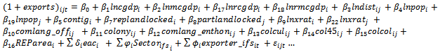
This study adopted with modifications, the Subramanian & Wei, 2003 extended gravity model specification. The modifications relate to dropping some covariates and including new ones not used in their study. Further, it replicates this approach for EAC using different products of EAC interest and different time periods of its formation. The general specification is of the following form;

(4)

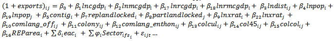
3.2. Specification of the Empirical Models

Following Carrere (2006) and Subramanian & Wei (2003), the above analytical framework is decomposed to the following specification:

(5)

Where expected signs:

The above equation was run to answer four research questions. The first question relates to estimating the effect of the adopted trade liberalization policy and determines which covariates explain bloc trade, especially the EAC dummy covariate, at the region and country levels? A priori, the signs on the dummies may not be determined. The expected signs of the other covariates are determined in other sections of the paper. The second question is to what extent did the EAC trade liberalization efforts affect its intra-bloc trading patterns of the selected sectors? A priori, the expected change is positive because it is widely believed that the formation of EAC and its membership marked a watershed in the status of EAC trading. This question is modified when counterfactual trade is included, i.e., including other members who normally trade as EAC though they are not formally members. And the key proposition the study addresses under this was whether EAC membership has a differential impact for the sectors chosen. And the food sub sector was used as a base dummy. The third issue is estimate the impact of EAC trade liberalization on intra-regional, export and imports of trade and hence implication on trade creation and trade liberalization? And fourthly, how is the trade liberalization effect distributed across each country? However, to estimate or analyze the distribution on the five EAC member states, equation 5 is modified for all the five countries.

3.2.1. Variables, Coefficients and Variable Definition

The cofficients embedded in these models include the β, δ, ϑ and ϕ coefficients estimates from the normal gravity model covariates, EAC dummies, sectoral dummies and exporter country dummies respectively. They show the major effects of each covariate on the exports.

The EAC dummy is specified in three forms, following Egger, 2002 and Soloaga & Winters, 2001 to formulate a correct ex-post assessment of the effect of the volume of trade, namely;

a. To capture intra-bloc trade, a dummy of both-in where δ is equal to one if both partners belong to the same RTA and zero otherwise, is introduced.

b. To capture bloc imports from the rest of the world, a dummy equal one if importing country j belongs to the RTA and exporting country i belong to the rest of the world, and zero otherwise, is also introduced.

c. And another dummy capturing bloc exports to the rest of the world equal to one if exporting country i belong to the RTA and importing country j belongs to the rest of the world, and zero otherwise is also introduced.

If the intra-bloc trade it means that intra-bloc trade has increased more than predicted by the reference which can be in substitution to domestic production or to exports from the rest of the world. As to whether this corresponds to trade creation (TC) or trade diversion (TD), one needs to examine the sign of the coefficients Trade is diverted when 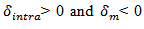(indicating a low propensity to import from the rest of the world), and when this negative propensity to import from the rest of the world entirely offsets the intra-bloc trade enhancement, this is pure trade diversion. However, when intra-regional trade increases more than imports from the rest of the world decreases, there is both trade creation and trade diversion. In this case, if and this is a case of pure trade creation. According Carrere, 2004, inference on welfare to non-members could be deduced on comparing the coefficients and That is, welfare is decreased for non members when and which indicates a dominant export diversion. So then, trade is purely created when and when also And trade is purely diverted when 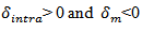when also The is a normally distributed random term that has a zero mean and a constant variance. And the other component of the model is the 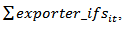capturing country effects or the component the EAC trade liberalization that is absorbed by each country. Sectoral dummies relate to the five sectors which were selected for this study. The food sector is the base category sector or reference sector. It’s the sector upon which the description of the sectoral dummies is discussed.

3.2.2. Types and Sources of Data

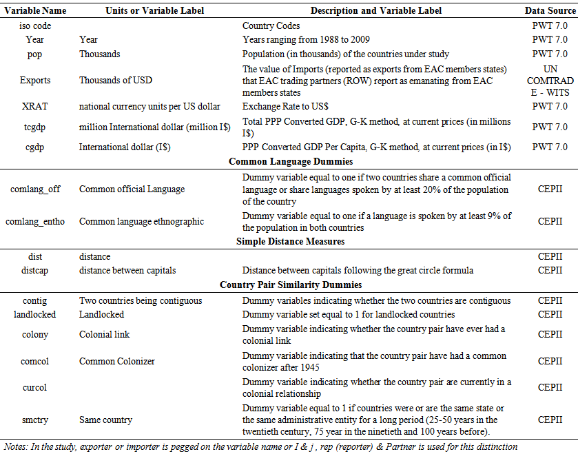
Gravity modeling and its estimations require data on bilateral aggregate trade, incomes, population, distance, as well as geographical, cultural, and historical information. The study uses a panel data set covering five (5) products (see appendix C Table 3.1) and one hundred sixty eight (168) importers who have indicating their trade with the five (5) EAC countries (Kenya, Tanzania and Uganda that acceded in 2000, and Burundi and Rwanda that joined in 2007; the study called these countries exporters). The list of countries (Exporters and Importers) used in the sample is presented in Appendix - D Table 3.3. The exporters are the members of the EAC community.

The study used secondary data from three main sources (see Table 3.2 in appendix B). The Trade data was mined from the UNCOMTRADE – WITS data base. The trade data used is unidirectional, that is, exports of EAC Partner States to the Rest of World (ROW). The use of the unidirectional (or imports of j from i) trade volume as the regressand (Subramanian and Wei (2003)) are due to: the fact that, theoretical specifications of gravity-like models yield predictions on unidirectional trade rather than total trade; secondly, the trade effects of trade liberalizations (such as WTO, GSP etc.) are closely related to imports rather than exports. The logic is simple, if country j liberalizes through a certain scheme like WTO or GSP with country i, it is expected that its imports from i would increase. However, there is no valid theoretical argument for its exports to expand by the same proportion even if the Abba Learner Symmetry holds; Abba Learner Symmetry states that the removal of import barriers serves to raise exports as well as imports. The symmetry would hold at the country’s aggregate trade level rather than at the bilateral trade level. And thirdly, the effect of a liberalization and elimination of export subsidies are ambiguous in theory, since an elimination of exports subsidies tends to reduces exports.

The second component of the data was mined from the then current Penn World Tables 7.0 (PWT 7.0). The Penn World Table (PWT) displays a set of national accounts economic time series covering many countries. Its expenditure entries are denominated in a common set of prices in a common currency so that real quantity comparisons can be made, both between countries and over time. It also provides information about relative prices within and between countries, as well as demographic data and capital stock estimates. From this table, I downloaded data on the following variables; Population (in thousands), Exchange Rate, Real Gross Domestic Product per Capita, current price, Price Level of Gross Domestic Product, Openness in Current Prices, Real GDP per capita (Constant Prices: Laspeyres), derived from growth rates of c, g, I, Openness in Constant Prices, and years for the period.

The third component of the data, was mined the from CEPII database. The data in this database relates to countries and their main city or agglomeration. Among the country-level variables are the first 3 identification codes of the country according to the ISO classification, the country’s area in square kilometers, used to calculate, in particular, its internal distance. Variables indicating whether the country is landlocked and which continent it is part of are also included. Also, I chose several language variables to proxy for indexes of language proximity or dummy variables for common language in dyadic applications like gravity equations. The sources for all language information are the web site www.ethnologue.org and the CIA World Fact book. For each country, a report of the official languages (up to three), as well as the languages spoken by at least 20 percent of the population and the languages spoken by between 9 and 20 percent of the population (up to four languages in each of those cases) was mined. Colonial linkage variables which were used are also often used by economists to proxy for similarities in cultural, political or legal institutions. Our dataset provides several variables (based on the CIA World Fact book, and the Correlates of War Project run by political scientists, available at cow2.la.psu.edu) that identify for each country, up to 4 long-term and up to 3 short-term colonizers in the whole history of the country.

4. Presentation and Discussion of Empirical Results

4.1. Descriptive Statistics

For any plausible study to be meaningful and the estimated model to have robust estimates it should begin by the description of the data and the estimated model adopted for the study. The description of the model relates to whether the covariates explain well the flow in exports. And the description of the data relates to finding out whether data is contaminated with outliers and influential variables. Where they were detected, they were treated as shown in the subsequent sections.

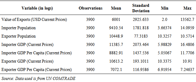
4.1.1. Summary Statistics

In this section, the summary statistics are presented and discussed. In the study, a number of covariates were used. However, Table 5.1 below presents the summary statistics for the major covariates used in the study.

From table 4.1 above, average annual trade value is about 6,000 in thousands of USD and this value could range between 2 thousand of USD and 14,000 of thousands of USD. The average population of the exporting countries of EAC is almost ten times the average population of the importing countries in the rest of the world. On average EAC has a population of about 10, 500,000 while the ROW has only 1,000,000 persons on average. The average nominal GDP and GDP per capita of the importing countries is more than 1,000,000 than that of the exporting EAC countries. The average GDP of EAC is 10, 603, 2000 and that of the ROW is 11, 385,700. While the per capita GDP is of EAC is 8,882,910 and the one for the ROW is 11,448,900 on average.

Table 4.1. Summary Statistics for Covariates used in the study

Table 4.2. Showing Correlation of Selected Covariates of the Study

4.1.2. Regression Correlation Matrix

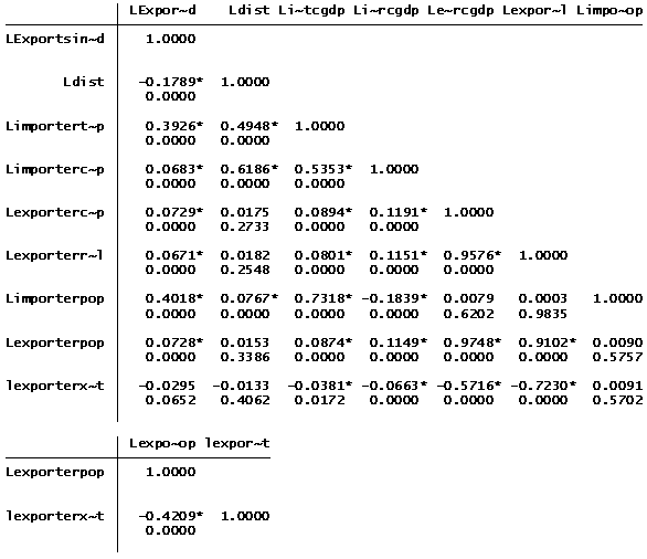
In order to find out the degree of linear relationship between the dependent variable (log of exports) and its covariates, a tabulation of the Pearson Correlation Matric was done. Table 4.2 below presents the correlation matrix for all the variables used in the model at the 0.05 level of significance.

The numbers in the table are Pearson Correlation Coefficients and move from positive 1 (implying a strong correlation) to negative 1 (implying an inverse relationship). All the variables are correlated with LExports in 1000s of USDs since they are all significant. The log of distance and exchange rate of the exporter are negatively correlated to the LExports as expected from theory. All the other variables have the expected signs of correlation to LExports. This implies that the covariates have a relation with the independent variable.

4.2. Assessment of the Model Using the Observed Versus Predicted Values

Another issues to consider before estimating the model, is to find out whether the predicted or specified model’s covariates predict the dependent variable (Lexports) well. To conclude on how well or good the model can predict the flow of exports, one looks at the relationship of linearity of the model and the behavior of its residuals. A graphical portrayal of this relationship is presented in Figure 4.1 below;

A visual inspection of the above figure indicates or shows the scatter producing a cluster of the relationship between the observed and the predicted values at a 45 degree pattern of the dataset. Because of this pattern, the model does a good job in predicting the exports of EAC.

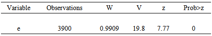
4.2.1. Test for Normality

Since this study used ordinary least squares to predict and produce its estimates, a normality test of the residuals was done. When the residuals are not normally distributed, the validity of the t-test, p-values and F-test will all be influenced. To achieve or conclude on this, a kernel density for a graphic interpretation (See figure 5.3 below) and the Shapiro-Wilk test for normality were applied. For the Shapiro-Wilk test, a null hypothesis that the distribution of the errors is normally distributed is prescribed. When the statistic is significant, we reject the null that the errors are normally distributed. In this study, Shapiro-Wilk test produces a significant statistic (with Prob> Z = 0) since it is less than 0.05, hence the null hypothesis that the data is normal or comes from a normal population is rejected. The Kernel density in Figure 4.3 below shows that the probability density distribution and the outlay of the residuals are not almost perfectly matching the normal distribution outlay. And when this is so, one concludes that the data is normally distributed.

Table 4.3. Shapiro-Wilk W test for Normal Data

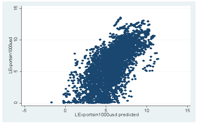Figure 4.1. Regression Results of Observed Against Predicted Values

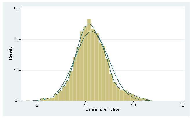Figure 4.2. Showing the Kernel Density Plot with an overlay of a Normal Distribution

Since in Figure 4.2 above, showing the kernel density plot not fitting the normal distribution plot perfectly, and Shapiro-Wilk test statistic being significant, it implies that estimates of the p-values, t-tests and f-test would not be valid and are even influenced. To overcome this problem, the dataset was transformed. The choice of the transformation was partly determined from theory and the use of the gladder commands of STATA.

4.3. Regression Diagnostics

Having determined, from the descriptive section, that the data, variables and model building processes are well-structured (or where they were not, they were corrected to be well structured), and that they behaved well in their relationship to each other and the dependent variable - exports, and in predicting the model, the study then did diagnostics test. The specific diagnostic test of Breush – Pegan for homoscedasticity and Wooldridge test for autocorrelation were done to check for and treat for heteroscadacity. The other diagnostic test related to finding out if the variables suffer from perfect multicollinearity or whether the errors are collated. Whenever the data suffered from these problems, then a solution for them was sought first before running regressions. However, when variables are perfectly collinear, then it is impossible to determine the determinant of the matrix used in transforming the variables, so as to assist in producing the estimates. And when the variables are autocorrelated, the estimates generated would be invalid since the t-values and standard errors would not be precise and efficient. If, the dataset does not suffer any of these or the problems have been accounted for, then the dataset and model may be used to estimate the results.

4.3.1. Testing for Homoscedasticity

In running the regressions, there was an important assumption that the variances of the residuals are constant or ‘homoskedastic’. To determine if this is so, a graphical method was used. STATA’s “rvfplot” inbuilt command was used to plot the graphical portrayal that helped in checking for homoskedascity. To reaffirm the graphical plot results, the Breusch-Pagan test was employed. However, without delving into the intricacies of these approaches, Stock and Watson 2003, notes that, ‘as a rule of thumb, always assumes homoscedasticity in your model’. Silva and Tenreyo, 2006, also allude to such a conclusion when they make mention of the fact that the null hypothesis that there is homoscedasticity is rejected in traditional fixed-effects gravity equations.

As such, this study presumed that the data suffered from heteroskedasticity. As such, the study predicted that the gravity model may provide wrong estimates of the standard errors of the coefficients coupled with wrong t-values. Since the results were estimated using STATA, one needs only to adjust the model by introducing the robust (re) option to the model to overcome this problem and improve the estimates of the regressions.

4.3.2. Testing for Multicollinearity

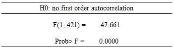
Another important assumption is that the independent variables should not be perfectly linear functions of each other. If they are, then it is not possible to find their determinants and hence solutions to the model are sought. However, in STATA, when variables are perfectly collinear, they are dropped automatically from the estimates. For example, the log of exporter GDP and GDP per capita variable have been consistently collinear in all regressions run. The current colony estimate was also collinear in all estimates. This is probably due to the fact that, there is no EAC member state that is in a current colonial relationship, hence the dummy variable’s determinant is not defined to help in the evaluation process of the estimate – causing the problem of perfect collinearity. As such, the variables were dropped from the estimation process by the statistical program.

The study also employed or used the Wooldridge test for autocorrelation in panel-data models. The test specifies a null hypothesis that there is no first order autocorrelation. When the test statistic is significant, then there is serial correlation. In Table 4.4 below, the Wooldridge test statistic is significant since its P-value is 0.000. And since this is less than 0.05, it implies that the null hypothesis is rejected. Hence, there is serial correlation or the model suffers from serial correlation.

Table 4.4. Wooldridge test for autocorrelation in panel data

Following Gurati, 2004, the study ignored the problem of collinearity since it does not seem to be serious and affecting the variables of interest. Only three variables were collinear and the explanation for this was established.

4.4. Summary of Econometrics Methods and Presentation of Results

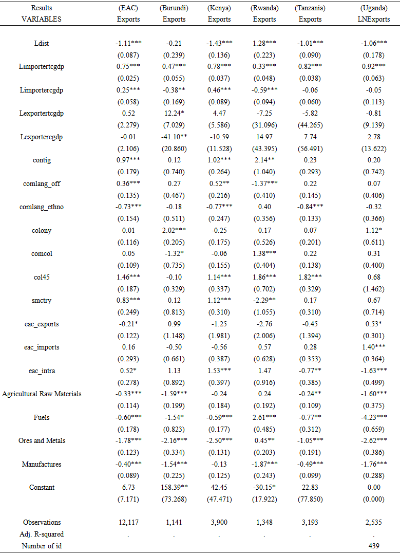
In the estimation of results, the following steps were followed with the justifications herein. Results relating to the EAC Bloc and that of the EAC countries are tabulated in Tables 4.5 in Appendix A. The tables showing the results of the different the econometric methods or models run with their appropriate statistical tests are not shown.

Empirical efforts of panel data often involves choosing between either running the within or squares dummy variables (called fixed effects model) on the one hand, and the generalized feasible (also called random effects). In this regard, a Hausman test was executed to decide on the appropriateness of the model to run. The Hausman test specifies a null hypothesis that the preferred model is random effects. While the alternative is that the fixed effects model is preferred. To achieve this, a fixed effects model i.e. run the ‘xtreg’ model with an option of fixed effects (fe) was specified and run with the results of the estimates stored. Then a random effects model was also run (i.e run the ‘xtreg’ model with a random effects (re) option and store the estimates). On specifying the Hausman test, it revealed a chi-2(15) = 235.72, which is highly significant at all levels. Because of this finding, the null hypothesis is rejected that the preferred model is random effects model. Hence the study employs the fixed-effects model.

The next econometric issue to consider was what type of fixed effects model to run and what estimation model to estimate. One could run the one-way, two-way and three-way fixed effects models. The choice of which at best, could partially depend on the data type and it size. However, trade data suffers from the problem of heterogeneity. Since heterogeneity was deemed and observed in the country pairs in the dataset, estimating a gravity model in panel eliminated this problem (following Westerlund and Wilhelmsson, 2006 conclusions). However, this would not eliminate all the heterogeneity in the trade data, especially emanating from the nature of the covariates. The study also took cognizance that estimates of the gravity model generated from a log-linear form using OLS are inefficient and not precise, i.e. they are biased and inefficient as Westerlund and Wilhelmsson, 2006 allude to and are not theoretically founded. Another issue confronting trade data and analysis is the presence of zero trade data which could be the result of no trade, measurement errors or rounding errors. Since trade data is normally in thousands of USD, the values which are less than half of this are rounded to zero, thus make estimate over- or –under estimated. To overcome this problem, the exports were measured not in thousands of USD but in their multiplicative form. Care was taken to avoid missing values. Where they existed; they were compensated for by exports, since the imports were the primary source of the trade data. And where the missing values still existed, they were considered to be true zero trade.

Since the traditional econometric method of estimating a gravity model in log-linearized form produces results that are not precise and efficient, the quest was to estimate a gravity model with a technique that handles the problem of zero trade data, solves the heterogeneity problem inherent in trade data, and is theoretically grounded. One of the only two theoretically grounded gravity estimation techniques, is to use the Poisson fixed effects estimator (pseudo Maximum Likelihood (ML) technique) in line with Silva and Tenreyro, 2006; and Westerlund and Wilhelmsson, 2006). The Poisson estimation was done with exports (the dependent variable) in it multiplicative form or original formulation not in a log-linearized form. The model was then estimated using OLS, producing better results that were not as biased and efficient estimates as those of the log-linearized gravity model. This is because the estimation procedure is done for zero trade, since the dependent variable is in level and it has no requirement for it to be an integer. The data was not Poisson distributed (Westerlund and Wilhelmsson, 2006). Therefore the Poisson fixed effects model, an appropriate estimation technique, was employed in estimating the gravity model. The estimates of this process are shown in table 4.5 in appendix A. Column one of table 4.5 shows results for the EAC bloc and the subsequent columns show the results for Burundi, Kenya, Rwanda, Tanzania and Uganda respectively.

4.4.1. Results of the Determinants of Exports of EAC

One set of objectives of this study was to estimate the effect of the adopted trade liberalization policy, determine and estimate which covariates explain bloc trade at both the regional and country levels. Having considered all the necessary econometric issues, a set of two equations were run and estimated.

Of the traditional gravity model covariates, the coefficients of distance, both the importer GDP and GDP per capita, sharing a common border, sharing official and ethnographic language, ever being in a colonial relationship and the trading country-pair ever being same country had positive and significant influences on trade. These and other covariates were all significant at 1 percent level and have the right signs theoretically, and as such, they determine the exports of EAC. For example, ceteris peribus, when there is a percentage change in distance, the exports of EAC decrease by 0.01. The impact is much smaller than the estimates generated by traditional OLS estimations of the gravity mode which is 1.12 (see table 4.5). However, EAC bloc exports going to a country sharing the same official language enhanced trade more than otherwise. This is because sharing a common official language enhances trade by 43 percent on average, more than the benchmark of exporting to a country that does not share this same language. However, EAC performance of exports going to a country sharing a common ethnographic language is not enhanced more than the benchmark. That is, sharing a common ethnographic performs less than not sharing a common ethnographic by an average of 52 percent. These findings seem to be in line with Silva and Tenreyro’s findings that distance and common language elasticities play a smaller role on trade for Poisson estimation than OLS estimations of the gravity model. The latter predicts an estimate on these variables closer to unity. However, a percentage increase in both the importer GDP and GPD per capita increase trade by 0.075 and 0.025 respectively. These estimates from ML estimations produce a greater effect on trade than those from OLS estimation techniques as asserted by Silva and Tenenyro, 2006. However, EAC exports going to countries that remained in the same colonial relationship after 1945, or to countries that shares a common border with it, and exporters who were the same country with EAC bloc, on average increased trade than otherwise by 331 percent, 163 percent and 129 percent respectively from the benchmarks.

More to this, Burundi’s exports are influenced by the choice of its importers’ GDP size and the fact that it has been in a colonial relationship with the importer. Ceteris paribus, for every percentage increase in the importer’s GDP, Burundi’s increase exports by 0.0047. Burundi’s exports are more enhanced when it exports to a country that has ever been in a colonial relationship with it than when it exports to one that has never been. This because, the colonial ties performs better than Burundi’s exports going to a country that has never been in a colonial relationship by 654 percent on average. The colonial ties also has similar effects on Uganda’s exports, i.e. when Uganda exports to a country that has been in a colonial relation with it, its exports are more enhanced because the colonial ties perform better than otherwise and on average it is 200 percent better than Uganda’s exports to country that has not ever been in a colonial link. The choice of the importer’s GDP also influences the exports of the other EAC member countries, just as Burundi’s. For instance, for every percentage increase in the importer’s GDP, the exports of Kenya, Rwanda Tanzania increase by 0.0078, 0.033 and 0.0082 respectively. However, a percentage increase in the importer’s GDP increases Uganda’s exports by 0.92 (which is closer to unity as predicted by theory). Another determinant that seems to influence most of the exports of the exporters or EAC states is distance. And for every percentage change in distance per kilometer, the exports of Kenya, Rwanda and reduce by 0.0143, 0.013 and 0.01 respectively. Nevertheless, Uganda’s percentage reduction in exports reduces by 1.06 for every percentage increase in distance.

Kenya’s exports are influenced by its own GDP, the GDP per capita of its importer, the contiguity of the importer of its products, the fact that its exports go to a country that shares the same official language with it, by the fact that it has ever been in a colonial relationship with the exporter and that they were the same country with the importer. For illustration, for every percentage increase in the GDP per capita of the importer and GDP of Kenya, the exports of Kenya increase by 0.005 and 0.12 respectively. But, when Kenya exports to a country it shares a border with, its exports are enhanced more than when it exports to one that is not in contiguity with it. This is because the contiguity out performs the lack of contiguity by 177 percent on average. Further, when Kenya exports go to a country that shares a common official language, it enhances trade more than when it exports to country that does not share this language. The reason being that, the common official language out performs the lack of it by 68 percent on average more than when it exports to a country that does not share a common official language. More to this, Kenya trading with a country that remained in a similar colonial relationship with it after 1945 out performs trading with a country that did not remain in such a relationship by 213 percent on average. Exports of Kenya are more enhanced when they go to a country that was one and the same with it, since same country within the last 75 years performs better than otherwise.

The exports of Rwanda are also influenced by contiguity of the importer of its product, i.e., contiguity enhances trade by 750 percent on average than not being in contiguity for Rwanda. Further, Rwandan exports are more enhanced when they go to an importer who has ever been in the same colonial relation after 1945 (col45) than when they go to a country that did not follow this arrangement. The col45 variable expands trade over 542 percent on average than not have exports go to such a country. While the col45 for Tanzania estimate of 517 percent overage outperforms the exports to a country which did not remain in the same colonial relation after 1945. However, the common colonizer indicator for Rwanda outperforms the exports to a non-common colonizer of Rwanda by 297 percent on average.

4.4.2. Application to the Assessment of the Effects of Regional Trade Agreements

Another objective related to finding the impact of EAC bloc on exports – especially its influence on trade creation and trade diversion and also imputes the welfare implications of the trade liberalization policy of the EAC trade agreement. To capture this, dummies of intra-bloc trade, bloc export and bloc imports were specified. Refer to table 4.5 for the estimates of these dummies. Inference is made for coefficients that are not only statistically significant, but also economically sensible. For EAC bloc, EAC_Exports and EAC_Intra dummies are significant. Following the Westerlund & Wilhelmsson, 2006 interpretation of these dummies, since the EAC_intra dummy coefficient is greater than zero (i.e. 0.05), it implies that the EAC bloc creates trade. EAC has created trade by 5 percent on average more than trade predicted by reference (it could be presumed to in substitution to domestically generated production). However, this statistic is lower than the 40 percent that is predicted from Poisson estimations. This lower figure could be due to truncating EAC importer members (to avoid homogeneity issues) and the truncation of the products used for analysis. However, since the coefficient of EAC_exports is less than zero (i.e. -0.21), then it is analogous to export diversion. This corresponds to export diversion of up to 19 percent on average. And following Carrere, 2006, since the EAC_Intra coefficient is positive and EAC_Exports coefficient is negative, this corresponds to pure trade diversion in terms of exports. This finding can also be used to infer on the welfare of the non-bloc members, i.e. the welfare of the non-members of EAC is reducing.

Kenya’s membership in the EAC leads to trade creation since the coefficient of EAC_intra is positive (1.53). The trade that is created by Kenya’s membership in EAC is about 361 percent than if it was not a member of EAC. In Tanzania’s and Uganda’s membership in the EAC however, seems to have reduced their trade creation effects since the EAC dummy coefficients for Tanzania of -0.77 and Uganda of -1.63, are negative, than the baseline. This corresponds to about 55 percent and 80 percent trade creation reduction on average than otherwise. Further, Uganda’s bloc EAC_exports is positive 0.53. This corresponds to 70 percent average reductions in trade diversion than explained otherwise. More to this, its estimate of EAC_imports and imports is positive 1.40. This corresponds to 306 percent analogous to reduction in imports diversion.

4.4.3. Application to the Sectoral Assessment of the Effects of the Adopted Sectors

The other objective of this study was to estimate the impact of EAC on food item trade in relation to the other sectors. A set of dummies capturing the sectors or product aggregates was specified with food sector as the base dummy.

The coefficient of the dummies for EAC sectoral trade in agricultural raw materials trade, fuels, ores and metals, and manufactures are -0.33, -0.60, -1.78 and -0.4 respectively. And since they are all negative, it means that the exports of the food sector perform significantly better than all the other sectors. For example, the performance of agricultural raw material exports is lower than the exports from the food sector by 28 percent for the bloc. More to this, the agricultural raw materials sector performs also less than the food sector in the rest of the EAC member states except for Kenya and Rwanda where the performance of the manufacturing sector is not significantly different from average contribution of the food sector on exports. The estimated coefficient for Burundi, Tanzania and Uganda are -1.59, -0.24 and -1.60 respectively. In terms of percentages, both Burundi’s and Uganda’s performance of agricultural raw materials on exports are on average 80 percent less than the food sector. And Tanzania’s agricultural raw materials average contribution on exports is 21 percent less than food sector’s performance.

The manufacturing sector estimates across all countries and EAC bloc outputs are all negative, implying that the sector performs worse than the food sector. However, the average performance of Kenya’s manufacturing sector on exports is not significantly different to that of food sector. The coefficient for the bloc manufacturing exports is -0.4, and that of Burundi, Rwanda, Tanzania and Uganda are -1.54, -1.87, -0.49 and -1.76 respectively. In percentage terms the manufacturing sector performance is comparatively worse than the food sector by 32 percent for EAC bloc exports, 79 for Burundi, 85 percent for Rwanda, 39 percent for Tanzania and 83 percent for Uganda. On the average, Rwanda’s fuel and ores and metals sectors perform worse than the food sector with coefficients of 2.61 and 0.45 respectively. In terms of percentages, the fuels and ores and metals sectors perform better than the food sector by 1250 percent and 57 percent on average in Rwanda. The fuels sector of EAC as a bloc and the rest of the EAC states perform worse than food sector too. At the EAC, the coefficient is -0.6, corresponding to a performance of 45 percent less than the average contribution of the food sector on exports. And for Burundi, Kenya, Tanzania and Uganda, the coefficients are -1.54, -0.59, -0.77 and -4.23 respectively. These correspond to average performances of 79 percent, 45 percent, 54 percent and 99 percent less than the food sector. A similar trend is observed for ores and metals. And the corresponding coefficient estimates of the Bloc, Burundi, Kenya, Tanzania and Uganda are -1.78, -2.16, -2.50, -1.05 and -2.62 respectively. In terms of percentage they are equal to 83 percent, 88 percent, 92 percent, 65 percent and 93 percent respectively.

5. Conclusions and Policy Recommendations

5.1. Summary of the Empirical Analysis

The study sought to answer three broad issues about the impact of the EAC adopted trade liberalization policy (or preferential trade liberalization or EAC trade agreement) on its partner states viz: the first question related to determining which covariates explain trade; the second, sought to estimate the effect on the sectoral trading patterns; and the third, was to assess the trade and welfare effects. An extended gravity model was run with a panel dataset extending 22 years (from 1988 to 2009). The dataset included 168 countries and five major products or sectors of EAC interest. The Poisson fixed effects estimation technique was used to run the gravity model for EAC, Burundi, Kenya, Rwanda and Kenya. Due to lack of convergence of Uganda’s trade data, its estimates were determined by the least squares dummy variable estimation. All the regressions were run using a two-way fixed-effects model.

For issue one, the study found out that the gravity model explained the trade pattern. And of the canonical gravity model covariates, the coefficients of distance, the importer GDP and GDP per capita , sharing a common border, sharing official and ethnographic language, ever being in a colonial relationship and the trading country-pair ever being the same country, had positive and significant influences on trade at the regional level. At the country level, the GDP of the importer positively influenced the exports of all the countries. Another covariate which affected (reduced trade) trade in all the countries except Burundi, probably because of its thin exports base, was the distance covariate. Trading with a country that remained in the same colonial relationship with EAC after 1945 influenced trade more positively than with a partner who did not. Burundi and Uganda’s exports responded more to trading with a partner who has ever been in the same colonial relation than if Burundi and Uganda traded with a country that had never been in the same colonial relation with them. Trading with a contiguous country benefited Kenya’s and Rwanda’s exports more than trading with a country that was not contiguous to them. Another positive influence was observed when the trading was with a country that was in a colonial relationship with it than with one which had never been in such an arrangement. Kenya’s exports are also influenced positively by size of its partners GDP per capita and its own GDP size. Furthermore, when Kenya trades with a country that was once the same country with it, and a country that use the same official language as it, it benefits more than trading with one that is otherwise.

For the second issue relating to the effect of EAC trade agreement on sectoral trade patterns with reference to the food sector, the study found out that:

• In the EAC bloc, the food sector performed better than all the other sectors – agricultural raw materials, fuels, ores and metals, and the manufacturing sectors. For example, in relation to the food sector, the agricultural raw materials sector, fuels, ores and metals and manufactures performance are 28 percent, 45 percent, 83 percent and 67 percent respectively.

• In Burundi, a similar pattern is observed in the food sector performs better than all the other sectors. The agricultural raw materials, fuel, ores and metals, and manufacturing sectors’ performance is 80 percent, 79 percent, 88 percent, and 79 percent respectively worse than the food sector.

• Food exports of Kenya performed better than all the other sectors of its exports. For example, the agricultural raw materials sector performed worse than the food sector by 21 percent. The fuels, ores and metals, and manufactures performed worse than the food sector by 45 percent, 92 percent and 12 percent on average.

• In Rwanda, it is only the manufacturing sector that performed worse than the food sector by 85 percent on average. However, the agricultural raw materials, fuels and ores and metals perform better than the agricultural sector by 27 percent, 1260 percent and 57 percent on average.

• In Tanzania, the food sector performed better than the other sectors that contributed to its exports. For example, the agricultural raw materials performed 21 percent worse than the food sector. The fuels, ores and metals, and manufactures sectors performance was worse than the food sector on average by 54 percent, 65 percent and 85 percent respectively.

• In Uganda, as similar to the performance observed in Burundi, Kenya and Tanzania in the performance of the food sector in relation to the other sectors. The agricultural raw materials, fuels, ores and metals, and manufactures sectors performed worse than the food sector by 80 percent, 99 percent, 93 percent and 17 percent respectively.

And for issue three, relating to assessing the effects of EAC trade agreement on the trade and welfare effects, the study found out that;

• The EAC agreement led to creation of trade at the bloc level of about 5 percent than otherwise.

• The EAC trade agreement led to a reduction in the welfare of non-members (rest of the world).

• Kenya’s membership to the bloc has enabled it to create more trade than if it was not a member. The trade created has expanded by 361 percent on average.

• Tanzania’s membership of the EAC bloc dampened it trade creation by 55 percent than if it was not a member.

5.2. Conclusions

The results of this study suggest that:

• The EAC trade liberalization policy reform that led to the formation of the EAC trade agreement has tremendously led to the growth and expansion of exports in all the sectors of food, agricultural raw materials, fuels, ores and metals, and manufacturing sectors. However, this growth is more reflective in the food sector on the one hand, followed by the agricultural raw materials and manufacturing sector on the other hand, more than the growth in the fuels and ores and metals sectors at the bloc level.

• Kenya is the biggest beneficiary from this growth, followed by Tanzania and Uganda, while Burundi and Rwanda were relegated beneficiaries but had a limp-frogging export growth.

• Intra-bloc exports increased tremendously across all the sectors. However, the manufacturing sector exports dominate the intra-bloc exports. The fuels sectors exports, though very small compared to the manufacturing sector exports follows in tow. This is closely followed by the food sector exports. The fuels and ores and metals sectors are also relegated to the much lower growth in the bloc too. It would be expected that since the food sector constituted the largest export growth without the bloc, it would also follow that it is the major intra-bloc export. However, this is not the case, since the manufacturing sector dominates intra-bloc exports. The reasons for the disparity of such an export outlay were beyond the coverage of this study.

• The choice of the importer mattered a lot in explaining EAC bloc exports. Importers of EAC export products that have large GDPs influenced trade more than those with trifling GDPs, ceteris paribus.

• Distance is an important factor in explaining the volume of exports from the EAC bloc. Proximate importers influenced trade more than detached importing countries.

• The implementation of the EAC trade agreement led to a creation of trade of more than 5 percent on average than that explained by the reference.

• The adopted EAC policy reform has led to an export diversion of about 19 percent on average than predicted by the reference.

• By inference, the implementation of the EAC trade agreement led to a reduction in the welfare of non-members (or the rest of the world).

• Kenya’s membership in the EAC and its implementation of the trade agreement led to Kenya creating more trade than was predicted by reference. The trade created by Kenya was about 361 percent on average.

• Tanzania’s membership and adoption of the EAC trade agreement reduced their trade creation by 55 percent on average than was predicted by reference or if it did not implement the trade liberalization mandate.

5.3. Policy Recommendations

The policy recommendations derived from these conclusions are:

• There is need to look at the structural components that hinder Tanzania and Uganda to create trade as a members of EAC. These hindrances possibly emanate from infrastructure inadequacies and NTBs to link Tanzania to its trading partners. The EAC Summit should strategize mutually to solve this by possibly introducing a trust fund to support especially the infrastructural limitations. There seems to be already and initiative to construct the Tanga-Mwanza Railway to link Dar es Salaam port to the hinterland to provide an alternative route and reduce on transportation expenditures, however, this has taken too long too. It is also recommended that such an initiative should be extended to link Burundi and Rwanda too.

• Minus Kenya, there is need for the other EAC members to build their export base and diversify the range of products they export (this is particularly recommended for Burundi and Rwanda). Where diversification is not tenable, the regional body should identify sectors that each country could specialize as its niche export sector, to avoid duplication of export sectors and enhance the exploitation of the available resources maximally.

• As the EAC is expanding in size, it’s important that the choice of its partners considered with economic rationale more than using the legal or political criterion. The EAC should in the medium term consider only accession partners with high GDP per capita, otherwise, those with low GDP per capita dampen the economic prospects of the bloc.

• In similar light, as EAC is busy looking for importers of its products, it is important that it sticks to importers who have high GDPs since they enhance trade more than those that do not ceteris paribus. It is also imperative that the partners to consider the proximity of the importer, the language they use both official and ethnographic, and their historical experience relating to colonization since these enhance trade more than considering importers who are otherwise.

• There is also need for EAC to develop a range of strategic policies to streamline the food and agricultural sector and their sub-sectors. The clouding and fusion of the food with other sectors should be separate, and let the food sector and possibly, other sector interventions not be synergized in a manner that will hinder their faster growth. This affects resource allocation, since the EAC may not know where to allocate it scare resources. It is recommended that the EAC could align peg it sectors after the WTO, such as the agreement on agriculture.

5.4. Delimitations and Suggestions for Further Research

An attempt to estimate the impact of myriad of aspects of a regional bloc like EAC in a single study like this is a daunting and unfeasible task. A study covering the wide range of details to fit such studies would necessitate rigorous and broad research. Further, it would require time, personnel and substantial costs. Therefore to produce a robust study that can be generalized, one has to make some delimitation.

Firstly, the study adopted gravity modeling to estimate the effects of EAC trade liberalization. Much as there have been marked improvements in its theoretical foundations, there are still disagreements on which type of gravity model to adopt and most times they do not fit the dataset quite well. As such, studies have found that the estimates of the gravity modeling are dependent on the covariates used and their number. For this reason, gravity modeling has a tendency to either underestimate or overestimate the weight of the estimates depending on the choice of covariates.

Secondly, the study uses a panel dataset of bilateral trade spanning 22 years for 168 countries. In using this type of dataset, there is a problem of attrition when the EAC member states cease trading with a partner or vice versa. Since the problem of the attrition in this data set seems to be completely random, the adoption of the data set should not be problematic. However, since EAC member states would concentrate on certain trading partners, and hence dropping the partners with limited trade dealings, the findings could give an impression that trading relationships are improving and profitable for those trading blocs (countries) than others, and further the concentration of trading with selective partners (the partners become non-random) with a large or significant trading with them. Besides this, span of the dataset used was purely influenced by availability of data for those countries in the databases. Availability of more years would provide more degrees of freedom to do a more robust analysis.

Thirdly, the study did not focus on inter bloc trade, rather on intra-EAC bloc trade. This can be conceived from the fact that, it does not include tariffs in its analysis. An inclusion of tariffs is expected to provide more valid estimates. However, tariff exclusion from the analysis should not negate the results of this study, since all the exporters in this study benefit from Special and Differential Treatment, and therefore the tariffs should not be expected to have a measurable effect on trade.

In addition, further research could seek as a methodological improvement to incorporate panel co-integration techniques and dynamic panel analysis unlike the static panel analysis that was adopted for this study. Panel co-integration techniques allow researchers to selectively pool information on country and product pairs regarding common long-run relationships from a cross the panel while allowing the associated short-run dynamics and fixed effects to be heterogeneous across different members of the panel under alternative hypothesis. In this way, the precision of the results is enhanced.

Appendix

Appendix A. Table 4.5 Estimation Results from Gravity - Table 1 Results of the Estimates of the Gravity Equation on Panel Data (1988 – 2009)

Appendix B. Table 3.2 Showing the Description of the Variables and Their Measurement

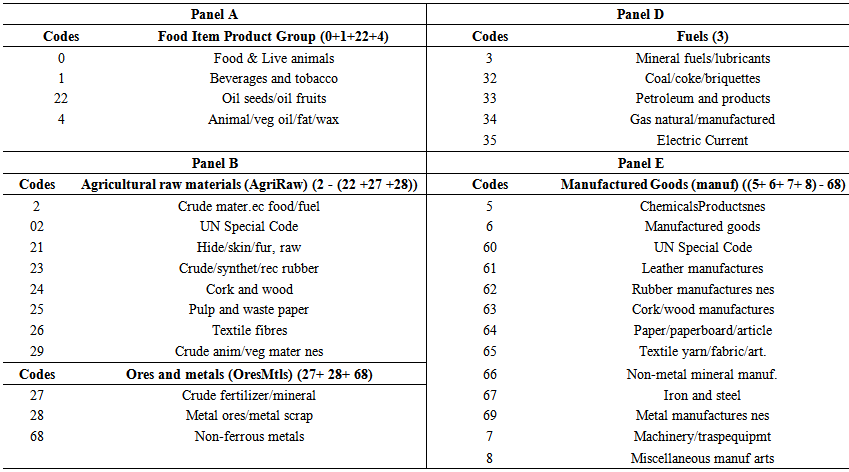Appendix C. Table 3.2 Composition of Products/Sectors using the SITC Revision 3 (1 to 3 digits)

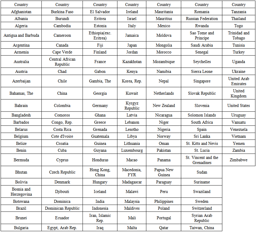Appendix D. Table 3.3 List of Importers of EAC Sector Products

Notes

1. Different, here means that, countries endowment of factors such of land, capital, labor and entrepreneurship are not the same in quality and quantity. And in production, a country with a larger and better endowment of these will have a cost advantage. As such, it will specialize in the production of that product, and this forms the basis of and gains from international trade.

2. Adopted from the following cite http: //benmuse.typepad.com/custom_house/trade_theory/

3. Cited from http://www.oppapers.com/essays/International-Trade-Theories/179424

4. Mercantilists policies are practiced at least by some firms doing business and it new supporters are known as ‘neo-mercantilists’ or ‘protectionists’ (Mahoney et al, 1998).

5. The exception to this (which is very rare), is when both nations have the same level of absolute disadvantage. In such a case, trade will not occur since there is no comparative advantage or disadvantage in the production of both commodities in both nations. In light of such intricacies, there was a need to reestablish the theory. That is, in the absence of equivalent levels of comparative advantage between trading partners for the products they trade, mutual and beneficial trade and exchange of trade in those commodities could take place when each of the said countries specialize in the production and exchange the products it has less absolute advantage.

The notion behind this is simple, because, when opportunity costs that differ between the countries but are constant within each country are considered for a factor, then the country with a lower sacrifice (opportunity cost) in that factor specializes in producing a certain commodity and exchanges it with the other country’s commodity, since the lower sacrifice enables it to have a comparative advantage in producing that commodity. Therefore, the difference in opportunity costs forms the basis for trade.

6. Cited fromhttp://www.marginalrevolution.com/marginalrevolution/2008/10/what-is-new-tra.html

7. Cited fromhttp://en.wikipedia.org/wiki/New_Trade_Theory. This period of time, the world experienced massive changes in structure resulting from the trade practiced adopted after the Second World War. For example, most countries synergized their industrials, sectors and policies by integrating. This new paradigm necessitated a formulation of new theories that endogenised pertinent issues of this new era like migration, transport costs, networks etc.

It has been argued that the only unique or new thing in the NTT was their mathematical rigor that included tacit use of protectionism.

8. Previous theories presumed perfectly competitive industries engaging in inter-industry trade (i.e. trading one product for another).

9. Ibid

10. Cited fromhttp://en.wikipedia.org/wiki/International_trade

• It is named after its analogy with Newton’s Universal Law of gravitation formulated as; 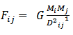where; F is gravitational force, M is mass and D is distance. That gravitational force between two objects depends on their masses and is inversely related to the square of the distance between them, all multiplied by a gravitation constant G (Keith 2003).

• The gravity model has been used to model many social interactions like tourism, migration, trade and foreign direct investment (FDI). They are econometric models which use ex-post analysis. And in trade, by design they are macro models since they are used to capture volume rather than composition of bilateral trade (Appleyard and Field 2001).

When it was introduced to trade by Tinbergen 1962, it had no theoretical foundation. He proposed that the same functional form (as seen above) that could be applied to international trade flows specified as;

(1)

Where; X are exports from I to j or total trade (it could either represent a flow from origin (i) to destination (j), or total volume of interruptions between I and j. Some authors like Rose, 2004 use average trade volume), Y economic size (proxies are gross domestic product or gross national income, Population); T is trade cost (proxies are distance, common language, colonial link, common currency, island or land locked). In the origin Newton model it is called distance. However in trade, we look at economic distance i.e. a sort of tax ‘wedge’ imposing trade costs, and resulting in lower equilibrium trade flows.

Model one above states that, bilateral trade between country i and j is inversely related to distance and positively enhanced by their sizes. The multiplicative nature of the gravity equation means that we can take natural logs and obtain a linear relationship between trade flows and the logged economy sizes and distances i.e.

(2)

The inclusion of the error term ϵ_ij in equation 2 above delivers an equation that can be estimated by ordinary least squares regression (OLS).

Deardorff (1998) was among the first persons to develop its theoretical foundation and he suspects ‘just about any plausible model of trade would yield something very much like the gravity model.’ Anderson and Van Wincoop (2003) too rein-enforced theoretical foundations and concluded in their proof that, ‘bilateral trade is determined by relative trade costs’. Other major contributions were by; Anderson 1979 when he emphasized the Armington hypothesis (i.e. goods differentiated by country of origin), Bergstrand 1990 when he considered monopolistic competition and price indices being those used in practice and not the ones suggested by theory.

11.

(6)

12. See table 4.1 in appendix 4.1 for details

13. See table 4.1 in appendix 4.1 for details

14. One may ignore this problem if the regressors are not perfectly collinear. This follows the “do nothing’ wisdom of Gujarati, 2004.

15. Wooldridge, J. M. 2002. Econometric Analysis of Cross Section and Panel Data. Cambridge, MA: MIT Press 282-283).

16. They state that biases and inefficiencies emanating from heteroskedasticity have been ignored in empirical work.

17. The upward rounding off could cancel the effect of downward rounding off and does not pose any problem. However, if your dataset included country pairs that are distant and even small this may not be plausible.

18. To generate exports, the study employed the multiplicative form i.e. Exports = Exportsin1000USD*1000 to generate an integer.

19. The imports were compensated or inflated by 10 percent (on average this is equal to CIF/FOB=1.1). However, there was also a pre-selection of the importers and exports used. Only exporters who had all the trade data for the period were considered.

20. When zero trade values still exist after these transformations and considerations, it should not be a problem when they are random. Nevertheless, this is not always the case. However, a serious problem will be encountered when the zero is in the dependent variable when the gravity model is estimated in it multiplicative form. Nonetheless, the gravity model (even in its log-linear form) can still be estimated with such challenges (Silva and Tenreyro 2006 & Frankel). And the challenges, especially of log-linearization, are even escalated in the presence of heteroskedasticity. As such, the estimates of the log-linearized gravity model are noted to be biased and inefficient and should not be used to infer trade dynamics. The traditional estimation of the gravity model involve one log-linearizing the model first and then estimating it with fixed-effects (Westerlund and Wilhelmsson, 2006). However, in the presence of heteroskedascity, the results of the OLS are biased and inefficient. Further, the log-linearized models truncate the negative trade and zero trade, or even some empirical the negative and zero trade are compensated for with a positive value. However, this introduces another problem of selection bias. There seems not to be a solution yet to handle zero trade however.

21. The other one involves using the two stage estimation technique developed by Helpman et al, 2007 that is identical to the sample selection bias. In the first stage, it involves finding the likelihood or probability that two countries trade with each other using the probit. This enables one to estimate the mills ratio. In the second stage, sing the mills ratio from stage one that controls for the bias in sample selection, and hence control for firm heterogeneity, and estimate the gravity equation in levels using the Heckman estimation technique.

22. The estimation results for EAC bloc were produced using the two-way Poisson fixed technique. The rest of the results were produced using the one-way Poisson fixed effects Poisson technique except for Uganda which were estimated the one fixed effect in it log-linearized form. This is because the results for Uganda failed to converge.

23. Carrere, 2004, quoting Obstfeld and Rogoff, 2001, suggest a consensus that the coefficient of distance should be between -1.2 and -0.8, which is identical to what is estimated.

24. Ibid