A. C. Akpanta, I. E. Okorie
Department of Statistics, Abia State University, Uturu, Nigeria
Correspondence to: I. E. Okorie, Department of Statistics, Abia State University, Uturu, Nigeria.
| Email: |  |
Copyright © 2015 Scientific & Academic Publishing. All Rights Reserved.
Abstract
In this paper titled ‘ On the Time Series Analysis of Consumer Price Index data of Nigeria -1996 to 2013’, the monthly CPI data collected from the CBN website was used. Although Time Series approach was adopted in the main analysis of the data, descriptive statistics of the data showed, inter alia, that the indicator has neither fallen below 21.19 nor risen above 152.29 within the specified period. A Seasonal Auto Regressive Integrated Moving Average (SARIMA) model of best fit to the data was discovered to be SARIMA (1, 2, 1) (0, 0, 1)12. Forecasts were made using the model and a t- test for the difference of two means of the forecast and the observed CPI values was carried out at 5% level of significance. Interestingly, the test shows no significant difference between the two.
Keywords:
Consumer Price Index, Time Series, Stationarity, Seasonality, ARIMA
Cite this paper: A. C. Akpanta, I. E. Okorie, On the Time Series Analysis of Consumer Price Index data of Nigeria -1996 to 2013, American Journal of Economics, Vol. 5 No. 3, 2015, pp. 363-369. doi: 10.5923/j.economics.20150503.08.
1. Introduction
A Consumer Price Index (CPI) measures changes in the price level of a market basket of consumer goods and services purchased by households. It is one of the several price indices calculated by most national statistical agencies. In Nigeria, for example, the National Bureau of Statistics is vested with the responsibility and is usually assisted by the Central Bank of Nigeria. The importance of CPI to any nation cannot be over emphasised. This is because it can be used to index the real value of wages, salaries etc. More so, it is one of the most frequently used statistics for identifying periods of inflation and deflation. No wonder, in 2006, Iwueze and Akpanta [1] did a stochastic modelling of inflation in Nigeria using CPI data. Inflation occurs with large rises in CPI during a short period of time while deflation sets in with large drops in CPI during a short period of time. In short, with information on CPI a country can gauge her economic health [2]. The CPI is computed using the Laspeyre’s method [3] where costs are computed using quantities from the base year.Following its relevance, most countries consider it as one of the national economic statistics to be closely monitored. It is therefore to provide a scientific base for this monitoring, modelling and possibly forecasting CPI values to guide investment and business plans and pricing [4] that a time series analysis of the CPI data (from 1996 till 2013) obtained from the CBN website [5] is undertaken.
2. Methods
The choice of time series analysis of the data was considered most appropriate since the data is indexed in time.
2.1. Time Series Analysis
Simply put, a Time Series is an ordered sequence of observations made sequentially in time. The most significant feature of such data is the likely lack of independence between successive observations in time. Time Series data can be univariate as in the case with the Consumer Price Index under consideration or multivariate.The ARIMA (Auto Regressive Integrated Moving Average) class of model is only reasonable for a univariate time series data. This method of time series modelling is also referred to as the Box-Jenkins modelling approach. ARIMA modelling technique could be traced to the work of Box and Jenkins 1976, [6]. With the ARIMA models forecast are made using the past of the process and are particularly suitable for short term forecasting and also forecasting seasonally enriched series. Box-Jenkins models are only reasonable for stationary time series with equi-spaced discrete time intervals. A good ARIMA model requires at least 50 observations and a reasonably large sample size is required for a seasonal time series [7].A time series is said to be stationary if its mean, variance and autocorrelation functions remain unchanged over time. However, in practice, many time series data are non-stationary and could be investigated by a statistically significant test e.g. the Augmented Dickey-Fuller test [8]. However, the problem of non stationarity could be addressed by a simple differencing exercise. Usually, the first difference is enough to coerce a non-stationary time series into a stationary one, and hence, the second difference is seldom required. Non-stationarity implies trend and is typically induced by serial correlation. Most time series plot that exhibit a fan like kind of fluctuation typically requires variance stabilization such as the Box-Cox transformation [9] before considering any data differencing.
2.2. Definition
Let  denote a non-stationary time series which could adequately be modelled by either a non seasonal ARIMA (p, d, q) model defined by
  | (1) |
or a seasonal ARIMA (p, d, q)(P, D, Q)s model defined by | (2) |
where  denote the order of the non seasonal and seasonal AR part of the model respectively,
  denote the order of the non seasonal and seasonal MA part of the model respectively,
  denote the number of times the non-stationary and seasonal time series needed to be differenced to stationarize and deseasonalize it respectively, and s in the seasonal model denotes the number of seasons. Interestingly, when
  , (1) and (2) reduces to ARMA (p, q) and seasonal ARMA (p, q)(P, Q)S, respectively where both are stationary process, defined by
  | (3) |
and | (4) |
respectively, where  are as defined above.
2.3. Non-Stationary Process
The random walk process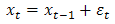 | (5) |
is an example of a non-stationary process, where  depends on the immediate past of the process and
  is essentially a stationary white noise process i.e.
  . Applying the first differencing to (5) we have
 | (6) |
Hence,  is a white noise process and stationary.
2.4. Steps to ARIMA Modelling
The ARIMA modelling approach entails to tentatively find a parsimonious model that describes the underlying generating process of the observed time series. However, the ARIMA model building consists of three steps: identification, estimation, and diagnostic checking steps. The identification step involves tentatively choosing one or more ARIMA model(s) based on the estimated ACF and PACF plots. The ACF plot of the AR (Auto Regressive) process decays exponentially to zero and its PACF plot shows cut-off at lag  and tends to zero afterwards. The ACF plot of the MA process shows cut-off to zero after lag
  while its PACF decays exponentially to zero. The combination of the AR (P) and the MA (q) processes is known as the ARMA (p, q) process (2) which has ACF and PACF that decays exponentially to zero. The maximum likelihood estimation method could be used in the estimation step to estimate the parameters of the identified model(s). The last step (diagnostic checking) involves assessing the validity of the identified and fitted model(s) through possible statistically significant test on the residuals to ascertain its consistency with the white noise process e.g. the Ljung-Box test [10]. Finally, the best fitting model would be selected among other competing models using the information criteria statistics on the basis of the AIC [11] and BIC [12] rule of thumb and forecast would be made using the model of best fit. Note that any out of the models with the smallest information criterion is the best.
3. Results and Discussions
A set of 18 years monthly Consumer Price Index (CPI) data from 1996 to 2013 obtained from the Central Bank of Nigeria (CBN) official website was thoroughly considered and analyses performed using R Statistical Software [13]. The results and discussions are presented below.
3.1. Descriptive Statistics
Table 1 shows some estimated summary statistics from which it could be seen that the CPI data used in this work has 216 observations and has neither fallen below 21.19 nor risen above 152.29 from January, 1996 to December, 2013. The first quartile (Q1) implies that 25% of the CPI is below the estimated value of 32.95 while 75% is above it. Analogously, the second quartile (Q2) or the median suggests that 50% of the CPI is below the estimated value of 60.66 while 50% is above it. Similarly, the third quartile (Q3) implies that 75% of the CPI is below the estimated value of 95.81 whereas 25% is above it. The mean implies that CPI would be 68.71 assuming the prices of all items remains the same across the period of study. The estimated variance of 1478.55 which is above twice larger than the corresponding mean value shows that the observations in the CPI data are further spread from the mean value. The estimated skewness and kurtosis statistics  imply that the CPI data are not normally distributed.
Table 1. Basic Statistics
 |
| |
|
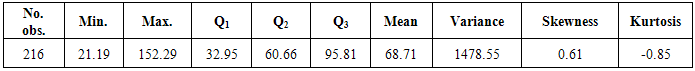
Next we present the ARIMA model building.  | Figure 1. From left to right: Time series plot, Auto Correlation Function (ACF) plot, and Partial Auto Correlation Function plot (PACF) |
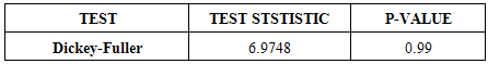
From Figure 1, the upward trend display of the Time series plot, the very slow exponential decay of the ACF plot, and the lag zero cut-off of the PACF plot suggest non stationarity of the CPI data. Also, the slight fluctuation in the time series plot appears relatively similar over time suggesting no variance stabilizing transformation such as the Box-Cox transformation. To verify the non stationarity of the time series as suggested by the plots in Figure 1, the Augmented Dickey-Fuller test was performed with hypotheses stated as follows:H0: The set of CPI data is unit root non stationary and H1: The set of CPI data is stationaryDecision: Large p-value 0.99 greater than 0.05 is in favour of the null hypothesis. Thus there is no evidence against the null hypothesis at 5% level of significance. Having visually shown from the above plots and a statistically significant test for stationarity that the CPI data is non stationary, it is now pertinent to transform the non stationary CPI data to a stationary time series by a trivial ordinary differencing so that the ARIMA models could be suggested.From Figure 2, the time series plot of the first ordinary differenced data shows somewhat periodicity (seasonality) in the first five years and thereafter a persistent violent fluctuation, both previously disguised in the trend, and accompanied by a slight upward trend which suggests non constant mean over time (non stationarity) in the data. This could be rendered stationary by a second ordinary differencing. The initial periodicity in the plot of the first ordinary differenced data and the upward trend are no longer observed in the plot of the second ordinary differenced data and the series fluctuates even more vigorously about a common value of zero suggesting stationarity after the second differencing. The ACF plot of the second differenced stationary series has cut-off at lag 1 and a pronounced spike at lag 12 (seasonal lag) also, the PACF plot has a cut-off at lag 11. However, these observations from the ACF and PACF plots suggest a Seasonal  for the non differenced CPI data.
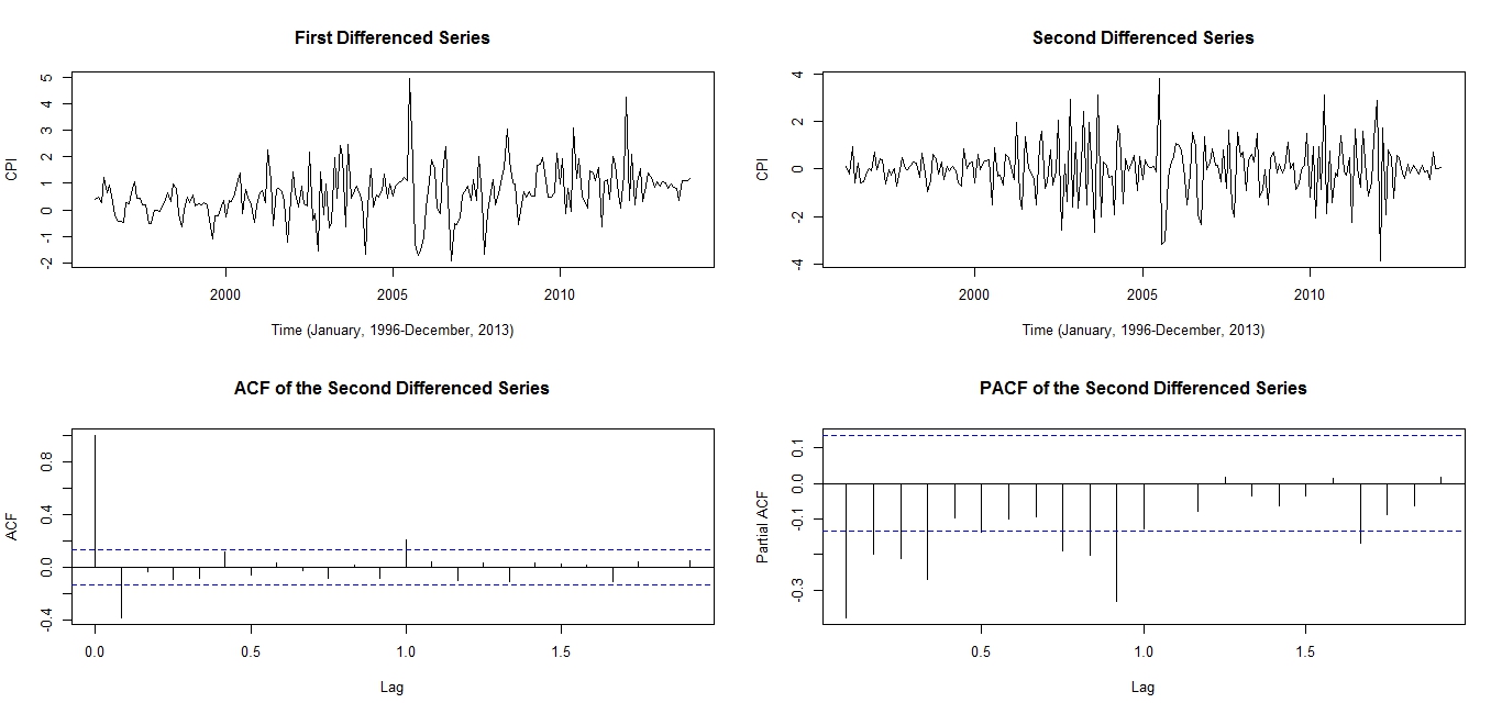 | Figure 2. First & Second Differenced Series; ACF & PACF of the Second Differenced Series |
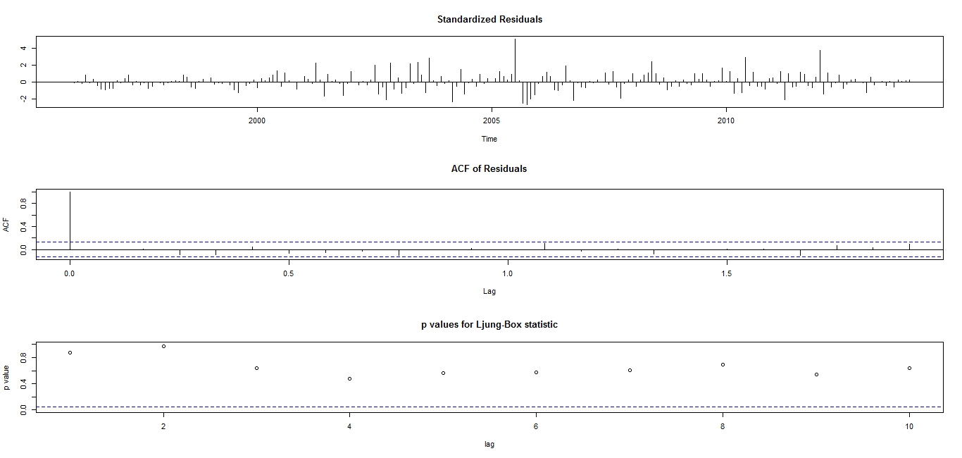
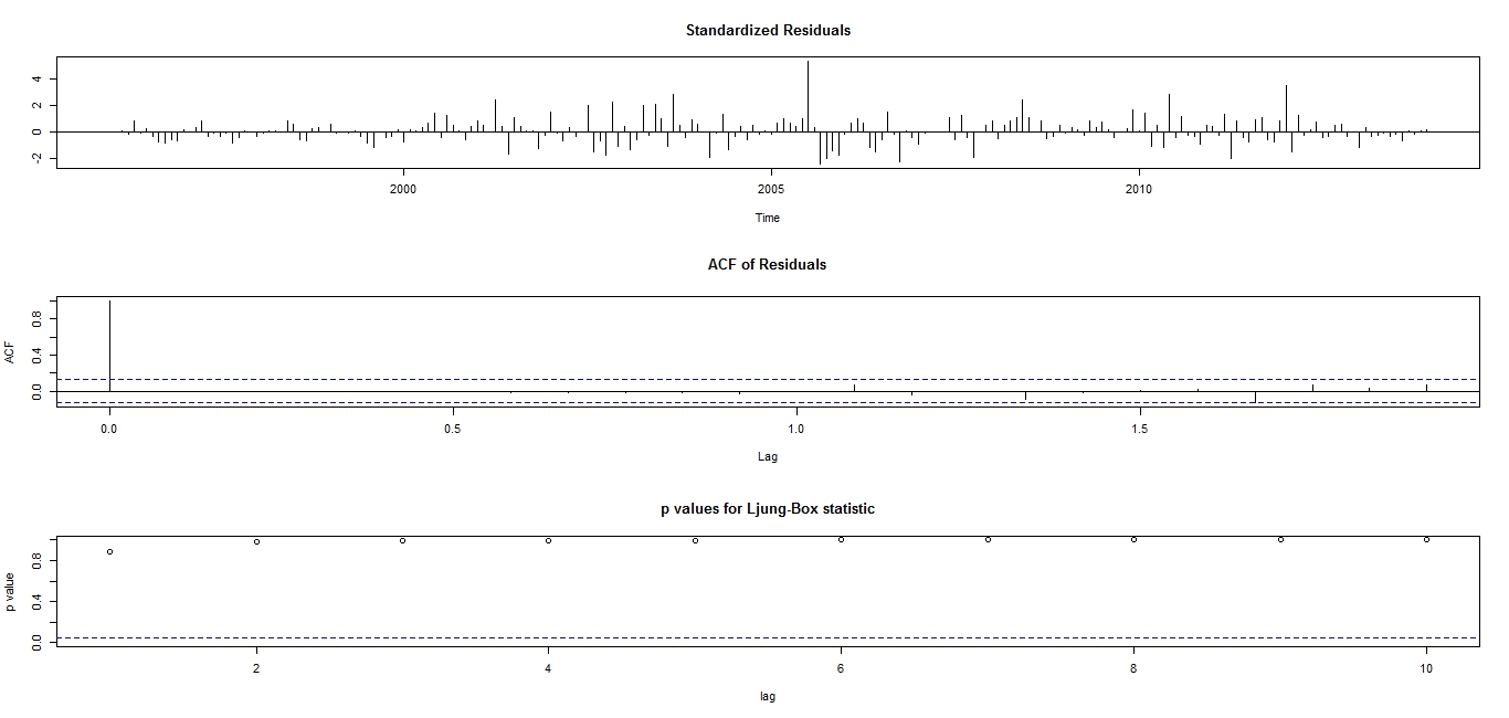 | Figure 3. Diagnostic Plots for the 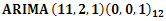 model model |
Based on the diagnostic plots, the 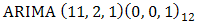 provides a good fit to the CPI data because the standardized residual plot swings about a common zero value and the points are evenly distributed on both positive and negative regions of the plot. The ACF plot shows that the Standardized residuals are uncorrelated at various lag points. The very large p-values of the Ljung-Box statistics lends more support to the uncorrelatedness of the standardized residuals. These observations from the diagnostic plots suggest that the standardized residuals of the fitted
  model are consistent with the white noise process. Although the diagnostic plots do not give any doubt on the adequacy of the fitted
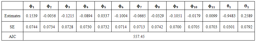
  model, the information in Table 2 shows the model to be over-parameterized and the following model parameters:
  and
and  are found redundant (not statistically significant). This is because their corresponding standard errors are more than twice larger than the estimated parameters. Tentatively dropping the non significant parameters and other intermediate significant parameters
  from the model we have a reduced and parsimonious Seasonal
  model for the non differenced CPI series.
Table 2. Augmented Dickey Fuller Test
 |
| |
|
 | Table 3. Fitted  model model |
 | Figure 4. Diagnostic Plots for the  model model |
The very small standard errors less than two times their corresponding parameter estimates in Table 4 suggest that all the estimated model parameters in the fitted  model are statistically significant. The diagnostic plots do not raise any alarm on the validity and adequacy of the fitted model because the standardized residual plot revolves about a common zero value suggesting no pattern in the residuals, the ACF plot does not show any spike above or below the 95% confidence bands (blue dashed lines) except at lag zero suggesting that the ACF of the residuals are uncorrelated at various lags. The very large
  p-values observed in the Ljung-Box statistics p-value plot does not say otherwise regarding the uncorrelatedness of the residuals at various lag points. Hence, the standardized residuals are consistent with the white noise process. The reduced and parsimonious
  model written in operator form
  with the smallest AIC statistics is preferred to the over-parameterized
  model given by
 therefore, is more suitable for forecast.
Table 4. Fitted
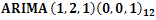 model model
 |
| |
|
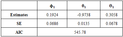
Observe from Table 5 and Figure 5 that there is a persistent increase and upward trend of the Nigeria Consumer Price Index. The heavy and light shaded region in Figure 5 corresponds to the 80% and 95% confidence bands, respectively, of the CPI forecast values. To validate the reliability of the forecast values, we perform a test on the difference between the means of the forecast and observed values using the Student's t-test. It is important to note that we have restricted the test to very few forecast values (January 2014 to July 2014) because long term forecast is not advisable for obvious reason.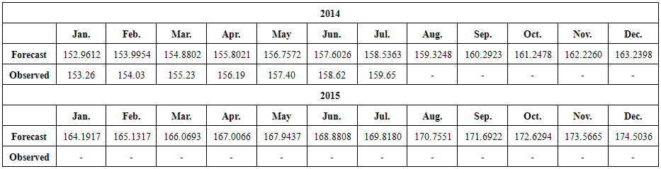 | Table 5. CPI Point Forecast Values and Observed values |
 | Figure 5. Forecast of Nigeria CPI from January 2014 |
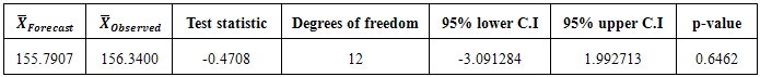
3.2. Test of Hypothesis on the Difference of Two Means of the Forecast and the Observed Values
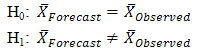 From the information presented in Table 6, we could reasonably conclude at 5% level of significance that there is no statistically significant difference between the observed CPI and forecast CPI values. This conclusion is made on the basis of the large p-value of 0.6462 which is greater than 0.05. Alternatively, it could equally be inferred from the 95% confidence interval (-3.091284, 1.992713) because the interval contains zero.
Table 6. Two sample t-test
 |
| |
|
4. Conclusions
The paper has examined 18 years data on Consumer Price Index (CPI) from 1996 to 2013 obtained in months from the CBN website. The basic statistics in Table 1 show, inter alia, that the indicator has neither fallen below 21.19 nor risen above 152.29 within the period under consideration. The major analysis was done using Time Series approach. The original plots, as well as the ACF and the PACF plots shown in Figure 1 suggest non stationarity of the CPI data and this was confirmed by the Augmented Dickey Fuller test summarised in Table 2. First and second order differencing were taken to coerce the non stationary data into a stationary one. Although the diagnostic plots carried out showed that ARIMA (11, 2, 1) (0,0,1)12 provides a good fit to the CPI data, the model seems to be over- parameterized hence the need to drop statistically insignificant ones became inevitable. This resulted to a parsimonious seasonal ARIMA (1,2,1) (0,0,1)12 for the non differenced CPI data as shown in Table 4. Forecasts were made using the model and a scientific comparison carried out showed that there is no significant difference between the observed and the forecast values of the CPI data.
References
| [1] | Iwueze I.S. and Akpanta A.C., 2006, Stochastic Modelling of Inflation in Nigeria. Global Journal of Mathematical Sciences, Vol. 5, No.1, 157-162 |
| [2] | McConnell C. R. and Brue S. L., 1986, Macroeconomics: Principle, Problems and Policies, 13th ed. McGraw- Hill Inc, New York. |
| [3] | Kapadia R. and Anderson G., 1987, Statistics Explained: Basic concepts and methods, Ellis Horwood Ltd, England. |
| [4] | Akpanta A.C., 2011, Statistics: The Steps Approach 1, 3rd ed. Rabboni Publishers Enugu, Nigeria, |
| [5] | http//www.cbn.gov.ng |
| [6] | Box G.E.P. and Jenkins G.M.,1976, Time series Analysis, Forecasting and Control. - San Francisco: Holden-Day. |
| [7] | Pankratz Alan, 1983, Forecasting with Univariate Box-Jenkins Models: Concepts and Cases: Wiley series in Probability and Mathematical Statistics, ISSN: 0271- 6356. |
| [8] | Dickey D. A. and Fuller W.A., 1979, Autoregressive Time Series with a Unit Root. Journal of American Statistical Association. Vol. vol.74. - pp. 427-431. |
| [9] | Box G. E. P. and Cox D. R., 1964, An analysis of transformations. JRSS, Vol. B 26 .- pp. 211–246. |
| [10] | Ljung G. M. and Box G. E. P., 1978, On a Measure of Lack of Fit in Time Series Models. Biometrika, Vol. vol. 65. - p. 297. |
| [11] | Akaike H., 1974, A New Look at the Statistical Model Identification. Annals of Statistics.: IEE Trans. Automat. Contr.,Vols. Ac-19. - pp. 716-723. |
| [12] | Schwarz G., 1978, Estimating the Dimension of a Model. Annals of Statistics, Vol. 6. - pp. 461-464. |
| [13] | R Development Core Team R, 2014: A language and environment for statistical computing. R Foundation for statistical computing. - Vienna, Austria ,3-900051- 07-0. |
 Abstract
 Reference
 Full-Text PDF
 Full-text HTML