1. Introduction

Economic growth, from the early period of economic history, engaged the attention of man and his governments. As far back as 17^th and 18^th centuries, writers like Adam Smith, David Ricardo, John Stuart Mill, as well as state theorist like Karl Marx, Friedrich List Karl Bucher, W Rostow, and neo classical economists such as Arthur Lewis (1978) [20] have all been preoccupied with the quest for unearthing the forces and processes that cause a change in the material progress of man. This is also applicable to successive governments and states in these modern times. In Nigeria for instance, the broad objective of the national economic policy has been the desire to promote sustainable economic growth for the vast majority of Nigerians through the adoption of various monetary and fiscal policies. Unfortunately, her economic growth performance has been characterized by fits and starts and the prospects of her rapid economic growth appear unachievable as reflected in her inability to realize sustainable full growth potentials and to significantly reduce the rate of poverty in the economy.

Several countries that have achieved rapid economic growth since World War II, have two common features. First, they invested in education of men and women and in physical capital. Second, they achieved high productivity from these investments by providing efficient capital markets, competitive trade-leading roles, higher level of economic efficiency driven by technological capabilities, stable polity, appropriate economic policy and economic system, World Bank, (2002) [29]. However, as a result of market failure that may likely occur in the process of development, it may not be ideal to leave the process of economic development entirely to the market forces especially in the developing economies like Nigeria.

Secondly, the quality of the government and its economic policies matter a lot. The radical theorist and the early proponents of development economics were of the view that growth could be internalized. Developments in the world economies have shown that it is futile for economies to isolate themselves from rapidly integrating world, Essien and Bawa (2007), [10].

Economic growth is a key policy objective of any government. In addressing the pertinent issues in economic management, experts and economic planners have had to choose between or combine some of the macroeconomic variables. Economic growth, proxies by Gross Domestic Product (GDP) confers many benefits which include raising the general standard of living of the populace as measured by per capita national income, making income distribution easier to achieve, enhance time frame of accomplishing the basic needs of man to a substantial majority of the populace.

Conversely, economic stagnation can bring destabilizing consequences on the citizenry, Lewis (1978) [20]. Controversies that trail growth-related issues are many, but the present and more incontrovertible is the discourse on economic growth within the context of macro-economic behavior of the economy. This is in relation to how the economic policy goals could be achieved by the available policy instruments. To date, the general consensus is that the rate at which declining economic growth rate is permeating the LDCs requires urgent policy response in order to bring about sustainable economic growth (Essien and Bawa, 2007) [10].

Furthermore, the Nigerian economy is basically an open economy with international transactions constituting an important proportion of her aggregate economic activity. Consequently, the economic prospects and development of the country, like many developing countries, rest critically on her international interdependence. Over the years, despite the considerable degree of her trade openness, her performance in terms of her economic growth has remained sluggish and discouraging, Odedekun (1997) [22]. Secondly, Nigeria’s trade policy since her independence in 1960 has been characterized by policy swings, from high protectionism to liberalism. The main objective of her trade policy is aimed at influencing trade process that can promote sustainable economic growth but this objective has become very difficult to achieve at present, Yesufu (1996) [30].

There is also an implicit belief that the Nigerian economic environment has been unable to attract foreign direct investment to its fullest potentials, given the unstable operating environment, which is characterized by inefficient capital markets, high rate of inflation, unstable polity, stringent policies and fragile financial system, among others.

Another major problem is the element of fiscal dominance. A size of fiscal deficit has an implication for domestic savings and investment and ultimately economic growth. In Nigeria, the main factor underlying these outcomes is the volatility of government expenditure arising from the boom and burst cycle of government revenue which is derived mainly from single export commodity (oil), whose price is also volatile. To worsen the problem, these expenditures are not channeled to productive sectors of the economy, Yesuf (1996) [30].

Prior to Nigeria political independence in 1960, agriculture was the mainstay of the economy. The present heavy reliance on primary commodity has induced adverse terms of trade shocks leading to huge current account deficits and exchange rate volatility and consequently a weak external sector for Nigeria. The trend in the current account amplifies the degree of import-dependence of the Nigerian economy. The deployment of the lean resources to finance huge debt service payments crowds out public investment in the productive sectors of the economy and with these developments, achievement of sustainable economic growth have become a difficult task.

Against this background of sluggish and volatile rate of economic growth which is accompanied with declining productivity signals, and Nigeria being a developing economy characterized by significant debt burden, structural imbalance and uncertainties, an insight into the determinants of Nigeria’s economic growth as well as their causal relationship with growth, has become pertinent.

However, most of the scholars of economics are of the view that the problem of Nigeria’s economic growth has not been well understood thus, improperly managed. Most of the reviewed studies have some methodological and conceptual problems that undermine their accuracy and thus their efficacy for effective policy purposes. For instance, non- application of unit root test to reduce or if possible, eliminate spurious regression due to non-stationary properties of the time- series and the use of cross-country analysis that precludes the country specifics, may all lead to biased inferences, Engel and Granger (1987) [8] and Gujarati (2009) [14]. Reviewed studies like Rogolf (2002) [25], Akintoby et al (2004) [1], Essien (2002) [9] and Essien and Bawa, (2007) [10], did not apply unit root test and some also applied panel and cross-sectional approach without taking into consideration the country’s policy differences.

Recognizing the above gaps and challenges of the previously reviewed studies, there is need to reexamine the problem of economic growth holistically by applying Nigerian time series using modern analytical econometric techniques such as Co-integration, Unit root test, Error Correction Mechanism (ECM) and Granger Causality tests, to see if a more authentic result could be achieved for effective economic planning.

Therefore the main objective of this study is to examine empirically the determinants of Nigeria’s economic growth by establishing the nature of relationship between economic growth and the selected growth inducing-indicators as well as establishing the nature of the direction of causal relationship that exists between them and economic growth. To achieve this objective, the following hypotheses are formulated to aid the analyses:

1. There is no long run significant relationship between economic growth (proxies by GDP) and some generally accepted economic growth determinants namely – productivity index (industrial), stock market capitalization, foreign direct investment, trade openness, savings, government fiscal deficit, and inflation.

2. There is no causal relationship between economic growth and the selected economic growth determinants.

The paper is structured as follows:

Section one which precedes four other sections introduces the study. Section two discusses the related reviewed literature. Section three provides the methodological issues. Section four presents and analyses the data while section five concludes the study with policy recommendations.

2. Review of Related Literature

2.1. Conceptual and Theoretical Issues

The term economic growth is described as the positive and sustained increase in aggregate goods and services produced in an economy within a given time period. When measured wit with the population of a given country, then economic growth can be stated in terms of per capita income according to which the aggregate production of goods and services in a given year is divided by the population of the country in the given period. Economic growth can also be stated in nominal or in real terms. Hence, when the increase in the aggregate level of goods and services is deflated by the rate of inflation, we have the real economic growth, otherwise when measured without deflating, it is called nominal economic growth.

However, the concept of economic growth has not been quite easy to grasp and measure in real terms. This is so because often on the literature of of economics, some authors have variously d differentiated economic growth from the rm “economic development”. For such authors like like Lewis (1978) [20], the mere increase in the aggregate level of production of goods and services in an economy tells us nothing about the “quality of life” of a citizenry, given the threats of global pollution, abysmal lop-sided distribution of aggregate output and income, environmental degradation, prevalence of chronic and deadly disease, abject poverty and the absence of freedom and justice. For such authors, attention should be focused not merely on the increase in aggregate output and income but also on the total quality of standard of living and that there is yet no satisfactory measure of “quality of life” that can be applied to quantitative measure of aggregate output and income which would be acceptable to all and sundry that will stand the test of the time.

Notwithstanding, the consensus appears to be that the term economic growth refers to a positive increase in the aggregate level of output within a given time period in a country while economic development is seen as sustainable increase in the aggregate level of output and incomes, with due consideration given to the quality of life which hopefully takes account of such issues as equal distribution of income, healthcare, education, environmental degradation, reduction in global pollution, freedom and justice etc. Therefore, economic development could be referred to as a process by which an economy experiences three main phenomena namely – sustained growth in output, structural changes and institutional changes, Woodford et al (2000) [28]. If these three phenomena take place, it will lead to a rise in standard of living of the populace. That is why growth could be enjoyed by many countries but not all experience development, Yesufu (1996) [30]. The term ‘economic growth’, is used throughout in this text to describe the positive and sustained increase in aggregate goods and services produced in an economy within a given time period.

Theoretical framework for understanding Economic Growth:

The framework for understanding growth over the long-term is rooted in two main theories that relates to possible sources of growth. These are the growth theory and the growth accounting theory. Growth theory is concerned with the theoretical modeling of the interactions among growth of factor supplies, savings and capital formation, while growth accounting addresses the qualification of the contributions of the different determinants of growth.

Three waves of interest have currently emerged in studying economic growth. The first wave is associated with the work of Sir F. Harrods (1900-1978) and E. Domar (1914-1997) in what was termed the “Harrods – Domar Model”. The theory presupposed that growth depended on a country’s savings rate, capital/output ratio, and capital depreciation. This theory has been criticized for three reasons. Firstly, it centers on the assumption of exogeneity for all key parameters. Secondly, it ignores technical change, and lastly, it does not allow for diminishing returns when one factor expands relative to another (Essien 2002) [9] and Woodford 2000 [28].

The second began with the neoclassical (Solow) model, which contained the thinking that growth reflected technical progress and key inputs, (labour and capital). It allowed for diminishing returns, perfect competition but not externalities. In the neoclassical growth process, savings were needed to increase capital stock, capital accumulation had limits to ensure diminishing marginal returns, and capital per unit of labour was limited. It postulates that growth also depended on population growth rate and that growth rate amongst countries was supposed to converge to a steady state in the long-run. Despite the modifications, the basic problems associated with the neoclassical thinking are that it hardly explains the sources of technical change (Essien and Bawa, 2007) [10].

The third is the newer alternative growth theory, which entrances a diverse body of theoretical and empirical work that emerged in the 1980s. This is the endogenous growth theory. This theory distinguished itself from the neoclassical growth model by emphasizing that economic growth was an outcome of an economic system and not the result of forces that impinged from outside. Its central idea was that the proximate causes of economic growth were the effort to economize, the accumulation of knowledge, and the accumulation of capital. According to this theory, anything that enhances economic efficiency is also good for growth. Thus this theoretical framework indigenized technological process through “learning by doing” or “innovation processes”. It also introduced human capital, governance and institutions in the overall growth objectives Romers, 1994 [26] and Essien, 2002) [9].

A number of endogenous growth is referred to in the literature as non-Schumpeterian growth. (Schumpeter emphasized the importance of temporary monopoly power as a motivating force in the innovative process). The model further incorporates the fact that technological advancement comes from what people do and existence of monopoly rents discoveries. The emphasis on knowledge and technology in the Schumpeterian model raises question about the role of government in promoting growth. Government should be seen as a critical agent that provides key intermediate inputs establishes rules, and reduces uncertainly, by creating the right macroeconomic environment for growth. (Contessi, et al 2009) [6].

The newer growth theory (endogenous theory) fits the real world perfectly well and has important policy implications. This is because it traces growth of output per capita to two main sources: savings and efficiency. In other words it is not only factor accumulation that drives growth but also efforts to utilize them. An important economic policy implication of this thinking is that of achieving economic stability with low inflation and positive (real) interest rate that spurs saving, which is good for growth, Contessi et al (2009) [6]. Consequently, anything that increases efficiency and savings is good for growth. This position is further examined in details in the subsequent section.

Endogenous Growth Theory:

Admittedly, some of the theories already discussed have helped immensely in explaining growth of individual countries but they do not completely explain why countries have differing growth trajectory. For instance, under the neoclassical theory, the long-run rate of growth in output was exogenously determined generally by an assumed rate of labour force growth. In other words, growth was traceable to a single source – technological progress, hence economic growth in the long-run was immune from economic policy whether good or bad.

The endogenous growth theory or the new growth theory, on the other hand, indigenizes the rate of technological progress. It traces the rate of growth of output per capita to two main sources – savings and efficiency. It also argues that policy measures can have an impact on the long-run growth rate of an economy, even if they do not change disaggregate saving rate. Thus countries with high level of efficiency, appropriate economic system, sound, economic policy, tend to grow more rapidly (Romer, 1994) [26]. Rapid growth rates are associated with country with efficient economic system and prestige (Lewis, 1978) [20]. This new thinking is very important for countries in an integrated arrangement or considering forming an economic union, and therefore aptly explains why countries economic growths are different ( Essien and Bawa, 2007) [10]

The efficiency argument is not entirely a new one. Economists have long held this view as they recognized technical change as important catalysts for economic growth. However, this endogenous growth theory is now being broadened to also include efforts to utilize the accumulated knowledge and other supportive conditions to optimal benefit. Thus technical change is viewed as an aspect of general economic efficiency. It is said to be good for growth as to squeeze out more output from a given input and that is what efficiency is about. Conditions that cause efficiency include education, diversification, privatization, liberalization, stabilization, strong capital market development etc. (Grossman and Helpman, 1991 [13] and Capasso, 2006 [3].

Education makes the labour force more efficient. Liberalization of prices and trade (trade openness) increases efficiency, stabilization reduces inefficiency associated with inflation, and privatization reduces inefficiency associated with state-owned enterprises.

Several authors like Akitoby et al (2004) [1] and Grossman, (1991) [13] have examined the role of technological progress or total factor productivity (TFP) in enhancing growth and have confirmed it to be a major explanation for the differences in economic performance across countries. It explains the poor growth performance of developing economies, especially the sub-Sahara Africa, and explained why the advanced countries have been getting richer. Reversing this trend, therefore, requires, finding innovations to raise total productivity, which in turn requires laying out proper conditions for thriving entrepreneurship in Schumpeterian sense, and increased foreign direct investment (FDI) in order to bring about structural changes in the economy. This is because innovation is seen as the main driving force behind economic growth and advanced and emerging countries are encouraged to attract FDI and other long-term flows through trade openness policy (Contessi et al 2009) [6].

However there is tendency in developing countries to seek to attract FDI without providing the necessary conditions for FDI to thrive. Some of these conditions include macroeconomic stability, fiscal discipline, strong and liquid financial system, minimal interest rate differential, flexible exchange rate management policy, robust external reserves, and fast growing GDP. Openness to trade without these conditions being met may be very costly. According Lederman et al (2003) [8] and Rogof (2002) [25], openness to international capital flows can be dangerous, if appropriate controls, regulatory apparatus and stable macroeconomic frameworks are not in place.

Further in explaining economic growth path, Economic system is defined as a prevailing economic ideologies, capitalism and socialism. All other types of economic system are mere hybrids or variants of these two. It can also be extended to include the degree of trade openness, trade regimes, and incentives. With regard to economic system, Romers (1994) [26] stated that the all- encompassing communism based on central planning and public ownership of almost all productive resources turned out to be a colossal failure wherever it was put into practice.

From his study of selected countries in comparable economic conditions and with much else in common (natural resources, culture shared languages but diametrically different economic systems), he found out that development was differed over a period of time. Thus, he concluded that economic factors, including economic systems, policies and institutions rather than exogenous technology, must have played an important role all along in determining the long-run economic growth performance of countries.

In addition, trade is an important and an integral part of an economic system. This is very important for growth, particularly in an integrated arrangement and the theory of economic integration is firmly rooted in trade theory. Lederman and Maloney (2003) [18] examined the empirical relationship between trade structure and economic growth particularly the influence of natural resource abundance, export concentration and intra industry trade, and found that regardless of estimation technique, trade structure variables were important determinants of economic growth.

Ayodele (2004) [2] in his studies found out that those countries that participated more in globalization through large increases in actual trade volumes since 1980 had increased growth rate. He found that while developing country’s growth rates have slowed down over the years that of the globalizing countries accelerated from the 1970s through 1980s to the 1990s. The increase in growth rates that accompanies expanded trade, therefore, on average translated in income. From the study, he concluded that open trade policy led to faster growth and poverty reduction in poor countries.

The economic policy argument emphasizes mainly on stable macro-economic environment as an important determinant of economic growth, although there may be other considerations like access to capital and social welfare of the numerous macroeconomic variables, inflation has been found to be a critical determinant of growth.

Hnatkovaska and Loayza (2004) [15] in their study investigated the relationship between macroeconomic volatility (inflation) and long run economic growth and found that they were negatively related. The negative link was exacerbated in countries that are poor, undergoing intermediate stages of financial development, institutionally underdeveloped, or unable to conduct countercyclical fiscal policy.

Another important issue under macroeconomic environment is the role of fiscal policy Tanzi and Zee (1997) [27] examined the relationship between public finance instruments and economic growth by surveying a large body of literature on ways in which taxes, public spending, and budgetary policy can influence growth. The authors concluded that fiscal policy could play a fundamental role in affecting long-run growth performance of countries by affecting allocation of resources, the stability of the economy, and the distribution of income. They recommend that changes should be made in the public finance instruments in the directions that theory has deemed important for enhancing growth, such as the adoption of policies to improve the neutrality of taxation, promote human capital accumulation, and less income inequality moreover channeling expenditure to productive sector to enhance private investment.

Studies have also shown that developing countries are often seen to be worst off when the macroeconomic environment is unstable. Akitoby and Cinyabuguma (2004) [1] investigated this view for a single country, particularly, the sources of growth in the Democratic Republic of Congo. Using a co-integration approach, the authors concluded that poor economic policies and conflicts, through their effects on total factor productivity and investment rate, significantly hurt the country’s economic performance.

In relation to direction of causality between openness to trade, foreign direct investment and economic growth, some studies like Lederman and Maloney 2003 [18] empirically established that causal relationship runs from trade structures to economic growth while Henriques and Sadorsky, (1996) [16], discovered that it is growth that leads and enhances export trade. Ogbulu (2009) [23], demonstrated that there is a feedback causality between economic growth and stock market capitalization.

Generally drawing an inference on understanding growth and its indicators there appear to be a general consensus from all the literature survey above that, overall, growth must be “endogenous” meaning that growth must respond to economic forces such as those released by different economic and political system or different economic policies. The major conclusions are that an economic system, such as central planning was bound to stifle economic efficiency and growth while a mixed market economy increases productivity. Thus, whatever a nation does to become more efficient will also help her grow more rapidly and thus these factors are regarded as its growth indicators or determinants. Romer 1994 [26].

3. Methodological Issues

3.1. Estimation Technique and Procedure

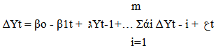
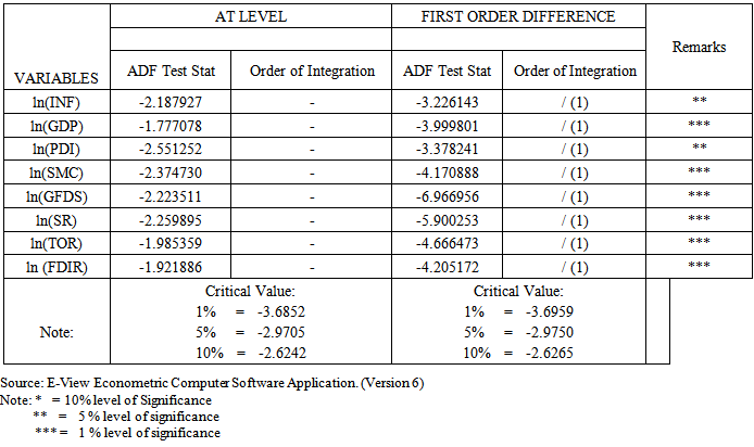
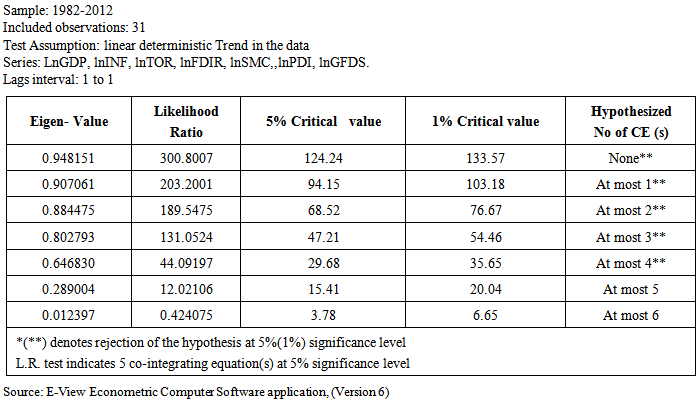
The study applied modern econometric analytical techniques namely - Co-integration, unit root test, Error correction mechanism (ECM) and Granger causality test for the data analysis, with time series secondary data obtained from CBN Statistical Bulletin, 2012 [5] and Annual Reports and Statement of Accounts 2012 [4] for the purpose of arriving at a dependable and unbiased analysis.

Prior to testing for the direction of causality, the level series OLS regression is applied at the first stage to test for long run relationship between growth and explanatory variables. However, being conscious of the characteristics of time series used, we are careful about the properties of time series used, there is need to be careful about the properties of stochastic error terms that might have entered the model which could give rise to spurious regression. Consequently, further rigorous investigations are made using ADF unit root test to check the stationary property of the variables (if any) in the model. The purpose of this test is to establish if the time series have a stationary trend, and, if non-stationary, to show the order of integration through ‘differencing’. A time series is stationary if the mean, variance and auto-variance are not time- dependent. The Augmented Dickey Fuller (ADF) (1981) [7] unit root test was applied. The assumption is that the time series used for this research have unit root stochastic process, represented as follows:

(1)

where Y is the single time series for ( TOR, FDI, INF, SMC, GFDS, SR, PDI and GDP) under investigation and β the parameter coefficient, ﻉt is a pure white noise error term, άi and גּ are coefficients of the lag terms and m is the length of the lag terms which is automatically selected using Akaike information criteria. If ‘גּ’ is 0, then there is unit root, but if it is less than zero (negative), the null hypothesis is rejected and the alternative that the series is stationary is accepted.

Capitalizing on the likelihood of a co-movement in their behavior which implies that there is possibility that they trend together towards a stable long run equilibrium, Johansen (1991) [17] Co-integration test is applied. The objective of this test is to determine if there is existence of long run equilibrium relationship among the variables used in the study. As pointed out by Engle and Granger, (1987) [8] the concept of co-integration creates a link between integrated process and the concept of steady equilibrium. Co-integration occurs when two or more time series variables which themselves may be non-stationary, drift together at roughly the same time. This implies that a linear combination of the variable is stationary. The null hypothesis is that the variables are not co-’integrated. Based on this, we specify the full information maximum likelihood based on the vector autoregressive equation (VAR) Johansen (1991) [17], as mathematically stated below:

(2)

where: yt is a k-vector of ‘differenced’ stationary time series, ‘k’ being the lag length for the first order differenced variables, /(1), ‘xt’ is a vector of deterministic variables, ‘a’ is a constant, ǿ are the coefficients of the deterministic variables and µ_t is a vector of innovations or error term and it is known as the adjustment parameters in the vector error correction model, while “t” indicates time dependent.. Using this method we estimated the equation in an unrestricted form and then tested whether we can reject the restriction implied by the residual rank of the co-integration.

Applying the maximal non-zero eigen -values and the trace test of the maximum likelihood ratio, with reference to the level of significance, the number of Co-integration relations could be determined which indicate the existence of long run relationship Johansen 1991. [17]

However, Co-integration process ignores the short run dynamics that might cause a relation not to hold in the short run and this formed the basis for application of Error correction mechanism (ECM). This is an extension of the partial adjustment model in co-integration technique which is the traditional approach to modeling of short run dynamics with long run equilibrium. It thus preserves the long run relationship while specifying the system in a short run dynamic way, Granger and Newbold (1977) [12], and Engel and Granger (1987) [8] are among the studies that have proved that a co-integration is a sufficient condition to run an ECM process. A vector error correction model is a restricted VAR (Vector auto- regression) that has co-integration restriction built into the specification so that it is designed for use with non-stationary series that are identified to be co-integrated. The co-integration residual term is known as the error correction term here, since the deviation from the long equilibrium is corrected gradually through series of partial short-adjustment, Gujarat and Porters (2009) [14].

A search for parsimony in this dynamic model typically follows the general–to-specific modeling (using various information criteria (Akaike, Schwarz, log likelihood, etc) which minimizes the possibility of estimating relationship while retaining long-run information, if the variables do not have the same order of integration, (Engel and Granger (1987) [8]. The functional form of the model, which initially is presented in a general form, incorporating many lag terms, is therefore later reduced to a specific or parsimonious structure by empirical testing and elimination and this gives the final and more precise result of the estimation.

Based on this, the specification is re-parameterize in a dynamic process and OLS regression applied with the equation as shown below:

(3)

Where a₀ is a constant, Y_t is a vector of endogenous variable and dependent variable, (GDP), Zi is a vector of explanatory variables and a_i is the parameter coefficients, Y_t-1 is the lag term of the dependent variable (GDP), the ecmt-1 or error correction term is the residuals from the long-run co-integration process and its coefficient measures the speed of the adjustment of the disequilibrium while μ_I is the white noise. As long as the co-integrating vector (ECM) ecm_t-1 is stationary and well defined, (negative), the ECM estimation will then confirm the earlier proposition that the variables are co-integrated or stationary. Equations 3, constitutes the maintained hypotheses for the ECM specification search. The insignificant or redundant variables are usually omitted at the parsimonious stage using Akaike Information Criteria and Schwartz Criteria. Finally, diagnostic tests are performed on the results with a view to validating the models.

Furthermore Granger causality test is used to determine if it is economic growth or the selected determinants are significant in either enhancing or deteriorating the rate of each other. It traces the direction of causality between economic growth and the selected growth determinant in Nigeria. To determine the direction of causality, the standard Granger causality test (1969) [11] was applied for this study. For instance, the test involves estimating a pair of regression as expressed below:

(4)

(5)

Equation 4 postulates that current GDP is related to each independent parameter (e.g trade openness) or their past values as well as its own past values (GDPt–j) where ά andβ are their coefficients, i and j indicate length of time lags while µt1 is the error term and n is the number of lag terms included. GDPt is the current value of economic growth (GDP).

In like manner, equation 5 postulates that current TORt) is related to a number of its lags ((TORt–i) or past values of itself as well as past values of GDP and the same explanations in equation 4 applies to equation 5. β,ά, фi and φ are the coefficients, and µ ₁ and µ ₂ are the disturbance terms, which are assumed uncorrelated, t indicates that the regression is a time series. The selected growth-indicators and GDP are the testable variables. 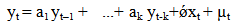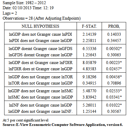For equation 4, the hypothesis that β = ά = 0 for all the ‘i’s, is tested against the alternative hypothesis that and . If the coeeficient β is statistically significant but coefficient ά is not, then GDP causes TOR. If the reverse is the case, then TOR causes GDP. However, where both coefficients are statistically significant, bilateral causlality exists. The same steps are applied to equation 5 and the remaining explanatory variables. The F- statistics ratios and their probabilities are used to confirm direction of causation based on the level of significance of the unrestricted OLS regression.

This approach is preferred to traditional correlation method that measures only the linear relationship which does not necessarily imply causation or direction in any meaningful word (Zellner, 1979 [31] and Granger, 1969) [11]. Usually three outcomes are possible – unidirectional when one null hypothesis is accepted and the other, rejected, bilateral or feedback when both null hypotheses are accepted and independence when none of the pairs of null hypotheses is accepted.

3.2. Analytical Framework

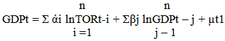
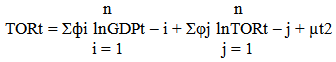
The analytical framework leans very closely to the newer endogenous growth theory prescription and extends the traditional growth accounting framework to focus on the variables which are Economic Growth (GDP) as dependent variable, Trade Openness, Stock market capitalization, Foreign Direct Investment, Productivity Index (industrial), National Savings, Government Fiscal Deficits and annual Inflation rate (assumed constraints) as explanatory variables. In accordance to this new growth theory, economic growth is determined by high level of savings and investments, economic efficiency, appropriate economic system and sound economic policy, among others, (Romer 1994) [26]. The endogenous growth model here is linear and could be mathematically written in both functional and natural-log form as stated below to make the analyses less tedious:

(6)

(7)

Where: Y = Economic growth (GDP)

TOR = Trade Openness (Export plus Import as ratio of GDP).

FDIR = Foreign Direct Investment (as ratio of GDP)

Inf. = Annual Rate of Inflation

SMC = Stock market capitalization (as ratio of GDP)

GFD = Government Fiscal Deficit

PDI = Productivity Index (Industrial)

SR = National Savings (as ratio of GDP)

U = Error term

Theoretical priori expectation: b2, b3, b5, b7 and b8> 0; b4 and b6<0.

Hence the above estimable long-run linear equation 7 posits that ‘Y’ the economic growth (GDP) in Nigeria is a function of (TOR), (FDI), SMC, GFDS, SR, PDI and Inflation rate. Economic growth (GDP) ‘Y’ is the dependent variable, ‘t’ indicates time dependent and µt is an unobservable component that is assumed “white noise”.

4. Empirical Findings and Analysis

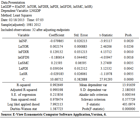
This section presents the data, the empirical results and discussions on the relevant findings from the model specifications tested in this study. Table 4.1 below shows the summary of empirical result when OLS multiple regression is run at the level series.

Analysis of the OLS Result

Table 4.1. Long-run OLS Regression (Variables measured at Level)

As presented on table 4.1above, the R-square (99.2) indicates ‘a good fit’ showing that 99 per cent of the variations in GDP are explained by the combined effect of variations in the explanatory variables. The F-statistics (405.09) confirms further that the explanatory variables are jointly and statistically important in explaining the variations in the growth process. These selected explanatory variables are correctly signed in accordance with the priori expectations except national savings with negative sign, indicating that savings is not contributing significantly to growth in Nigeria. The implication is that FDI, TOR, PDI, SMC enhances economic growth while inflation and GFDS are growth constraints in Nigeria.

However, a cursory look at the low D.W (1.3877) ratio and high R-squared (99.2) show possibility of first order positive serial correlation in the face of non-stationary properties of the times series variables regressed at level. This indicates some degree of time dependence of the series at level and this can lead to spurious regression. The variables are therefore re-examined using the ADF (1981) [7] unit root test.

Unit Root Test Result Analysis

Table 4.2. Summary of the Unit Root Test Result - Data Presentation

In line with recent development in time series modeling, unit root test is basically required to establish whether the time series have stationary trend, and if non-stationary, the number of times the variable has to be differenced (screened) to arrive at a stationary. This could form the strategy and reduce (if not eliminate) the risk of spurious regression, Engel and Granger (1987) [8] and Granger and Newbold (1974) [12]. Usually the test (using first or series of orders of ‘differencing’) fringes the variable to stationary if not stationary. As presented in table 4.2 above, the unit root test shows that the null hypothesis can only be rejected after the first order differencing /(1) for all the selected variables at one and 5 per cent level of significance. This is evidenced by ADF test result at the ordinary level, which shows that the computed negative ADF test statistics for each variable, is less than the Mackinnon (1991) [21] critical value in absolute term. Thus, the null hypothesis is accepted at level series indicating that all the variables are non-stationary at level but only became stationary after first order unit root differencing (screening).

Table 4.3. Summary of Johansen Co-integration Test Results - Data Presentation

ECM Result Analysis

The parsimonious ECM Growth model result presented in table 4.4 below gives the final and more precise estimation result when compared with the OLS level series model. All the variables are correctly signed as predicted and measured by their regression coefficients. The F- statistics ratio of 15.7 with probability ratio of 0.0002 confirmed that the explanatory variables (economic growth determinants) are jointly and statistically important in explaining growth nexus in Nigeria. The (R²) of 86 per cent displays overall goodness of fit and is also significantly high, implying that the changes in selected explanatory variables in aggregate, accounted for 86 per cent of the variations in economic growth (GDP) performance in Nigeria. GFDS is omitted in this short run process, implying that government excessive expenditure is only significant in the long run. However, TOR though positively related, has a weak impact as suggested by the size of its regression coefficients ( 0.002 lagged two periods) in part, implying that one per cent increase in TOR in part, induces only 0.002 per cent in the GDP growth rate in the long-run. Inflation rate has significant inverse relationship with GDP as predicted, implying that it is a constraint to economic growth in the long-run. Durbin-Watson statistic ratio of 2.3 indicates absence of serial correlation. This indicates that the unit root test has effectively screened the time series variables to achieve stationarity when compared with DW statistics (1.3) of the OLS level regression result.

Table 4.4. Summary of Parsimonious Error Correction (ECM) Model

The coefficient of the ECM term which measures the speed of the adjustment of the dependent variables at which equilibrium is restored, (-1.160) is significant and correctly signed (negative) at 5 percent level, and therefore confirms our earlier proposition that the variables are co-integrated. The speed suggests that economic growth in Nigeria adjusts slowly to the long-run equilibrium changes in the explanatory variables and it gives the proportion of the disequilibrium error accumulated in the previous period that is corrected in the current period. The speed implies that 16 per cent of any disequilibrium in the economic growth process is corrected within a lag (one year in this study).

This result is in agreement with Akitoby and Cinyabuguma (2004) [1], Odedokun (1997) [22] and Hnatkovaska and Loayza (2004) [15].

Pairwise Granger Causality Test Analyses

The above test as presented in table 4.5 was run on the model with optimal lag of 2. The essence of this test is to establish the direction of causal relationship between economic growth and its selected determinants. It is preferred to traditional correlation which measures only relationship without direction. Establishing which variable causes or promotes the other, will enhance effective economic planning especially in determining the relative weights to be assigned to these macroeconomic variables in achieving sustainable economic growth.

As presented in table 4.5 and capitalizing on the F-statistics ratios, there exists unilateral causal relationships between the economic growth (GDP) and some of the growth determinants (TOR and INF.) with F-statistics and probability ratios of 9.1829 (0.0045) and 5.2601 (0.01022) respectively at the 5 percent level of significance. This result suggest that inflation and TOR determine GDP without a feed back in Nigeria while significant bilateral causality runs between GDP and FDI as well as SMC with feedback implying that the variables determine each other. Independent causality exists significantly between PDI and GDP implying that it could not be determined which variable enhances the growth of the other.

Table 4.5. Summary of Pair-wise Granger Causality Test Results

The general results imply that causal relationship between economic growth and the selected determinants is mixed and therefore inconclusive.

However, it agrees with the findings of Pentecost and Kara (2000) [24] and Ogbulu (2009) [23] which show that causality tests are mixed and inconclusive depending on the variables used.

5. Summary and Conclusions

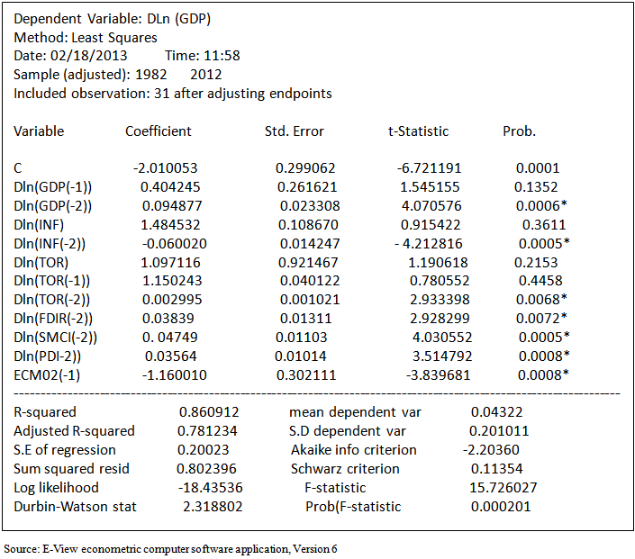
This paper examined the nature of relationship between economic growth and some selected growth determinants in Nigeria as well as the direction of causal relationships that exist between those determinants and economic growth, employing the Johansen co-integration, unit root test, Granger Causality and ECM tests, with data sourced from CBN Statistical Bulletin and Annual Reports, 2012, and drawn from selected annual key macroeconomic time series in Nigeria for a period of 33 years (1980 to 2012).

Based on the empirical evidence, using the newer endogenous growth framework, the study has brought to fore that the applied explanatory variables have a long run relationship with GDP and are major growth determinants. In aggregate, they explained significantly the variations in the economic growth nexus in Nigeria. Government excessive fiscal deficit and inflation with inverse relations are confirmed to be impediment to achievement of sustainable economic growth in Nigeria in the long run. The coefficient of the ECM term which measures the speed of the economic growth adjustment, suggests that economic growth in Nigeria adjusts slowly to the long-run equilibrium changes, with only 16 per cent of the disequilibrium in the economic growth process being corrected within a lag (one year in this study). This outcome also suggests a lag effect of the monetary policy instruments. However, trade openness, though positively related to GDP, has a weak impact on growth.

Over all, this study have examined several explanations for the pronounced fluctuations and sluggishness in Nigeria’s economic growth and confirmed that government fiscal indiscipline as well as volatile and persistent rise in price level are major contributing factors that have adversely influenced economic growth in Nigeria despite the positive impact of other determinants.

6. Recommendations

The significance of the findings obtained from the study poses a serious challenge to the economic and policy makers. Based on these findings, the study recommends that the government should strive to achieve sustainable price stability, stronger capital market with minimized distortions, fiscal discipline that channels funds to productive sectors to encourage private investors. Economic efficiency driven by infrastructural support and enhanced technological capabilities, strong institutional and economic reforms can increase production capacity. In addition, stable polity, to promote trade, domestic and foreign investments, should also be highly emphasized. There is also need for the policy makers to take cognizance of the policy lag effect and design policies in line with the expected magnitude of expected changes. Strategies for poverty eradication in addition to prudential and effective management of government expenditure can also lead to increased savings specifically through the oil revenue.

ACKNOWLEDGEMENTS

The author wishes to acknowledge and appreciate all those who in one way or the other, contributed immensely to the development of this paper, especially Assoc. Prof. Ogbulu, M. A of Abia State University, Uturu, Nigeria and Prof. Iheduru of Madonna University, Nigeria, for their time in vetting this work.