Logubayom Anuwoje Ida, Luguterah Albert
Department of Statistics, University for Development Studies, Navrongo, Ghana, West Africa
Correspondence to: Logubayom Anuwoje Ida, Department of Statistics, University for Development Studies, Navrongo, Ghana, West Africa.
| Email: |  |
Copyright © 2014 Scientific & Academic Publishing. All Rights Reserved.
Abstract
Macroeconomic variables are the main signposts signaling the current trends in an economy. Economic stability is desirable because it encourages economic growth that brings prosperity and employment. In this study, data on the 91-day Treasury bill (T-bill), 182-day Treasury bill (T-bill), inflation and exchange rates obtained from the Bank of Ghana from January, 2000 to October, 2012 was modeled using multivariate time series methods to investigate the dynamic interrelationships existing between them. The results revealed that, an optimal lag of one (1) should be included in the VAR process, therefore a VAR (1) model was fitted to describe the relationship between the variables. Results from the VAR (1) model, Granger Causality, Impulse Response Function (IRF) and Forecast Error Variance Decomposition (FEVD) analysis showed that; there exist a unidirectional relationship between the 91-day T-bill and 182-day T-bill rate, between the 182-day T-bill and Inflation rate, between inflation and exchange rates and between the two T-bill rates and exchange rate. Bothunivariate and multivariate Ljung-Box and ARCH-LM model diagnostics test performed on the residuals of the individual equations and the overall VAR (1) model revealed that the residuals were white noise series. The chi-square goodness of fit test performed on an out-sample forecasted growth rates of each rate showed that the VAR (1) model fitted was adequate for determining the behavior of the rates over time.
Keywords:
Dynamic relationship, Growth rate, Multivariate time series, Stability, Unidirectional
Cite this paper: Logubayom Anuwoje Ida, Luguterah Albert, Modeling the Dynamic Relationships between Treasury Bills, Inflation and Exchange Rates in Ghana, American Journal of Economics, Vol. 4 No. 5, 2014, pp. 200-212. doi: 10.5923/j.economics.20140405.02.
1. Introduction
Maintaining macroeconomic stability has been one of the major challenges for many developing countries. Factors such as market capitalism, interest rates, government stock rates, exchange rates, money supply, inflation in financial instruments among others, exert some impact on the development and growth of an economy [1]. A stable economy is characterized by the absence of excessive fluctuations in the macro-economy [2]. Economic stability is desirable because it encourages economic growth that brings prosperity and employment. Low inflation in a strong, well-managed area makes government borrowing less expensive and interest repayments on national debt substantially reduced. In addition, economic stability allows governments to plan national finances, expenditure and revenues with more certainty [3]. The instability in many economies persists over a long period of time because; much focus is not placed on studying the performance, structure, behavior and relationships among these variables over time. The governments, in order to macro-manage the economy well, must study, analyze, and understand the major variables that determine the current behavior of the macro-economy over time. A number of researches have been done in identifying linkages between some of these macroeconomic variables. For instance, Engle and Granger [4] formalized the concept of co-integration while Nguyen and Seiichi [5] found that the real exchange rate is an important macroeconomic instrument for ensuring low inflation rate and a stable financial system that promote exports, control imports, and enhance economic growth. Noer et al. Noer et al., [6] identified that, in the system of floating exchange rates, exchange rate fluctuations can have a strong impact on the prices of goods through the aggregate demand and supply. The weakening of exchange rate will raise the price of inputs, thus contributing to a higher cost of production and certainly increase in the price of goods that will be paid for by consumers. As a result, the price level aggregate in a country could continue to increase causing inflation. Goldfajn and Gupta [7] employed Vector Auto regression (VAR) modelling based on the impulse response function, to study the linkage between real interest rate and real exchange rate for the Asian countries and did not find any strong relationship between interest rate and exchange rate. In his study, Berument [8] found that inflation rate had a positive influence on the 91-days T-bill rate when he used conditional variance of inflation rate to represent risk index. Luguterah and Logubayom [9] modeled the relationship between the Ghanaian T-bill, inflation and exchange rates using the co-integration approach. Their results revealed that, these set of variables were co-integrated and two linearly independent co-integrating equations described the equilibrium relationship between the time series variables. Even though Treasury bills (T-bills), inflation and exchange rates are recognized in many developed and developing countries, including Ghana, as economic impacting factors, there are limited researches in the Ghanaian economy on how these variables interactively affect each other over time as a result of changes in one or more of them. This study therefore used historical data on the 91-days T-bills rate, 182-days T-bills rate, inflation rate and Exchange rate from the Bank of Ghana to investigate the dynamic relationship between growth rates of these variables by employing multivariate time series techniques such as the Vector Autoregressive modeling (VAR), Granger Causality, Impulse Response Functions (IRF) and Forecast Error Variance Decomposition (FEVD) analysis. This study gives an idea of how these rates interact among themselves over time and how each macroeconomic indicator serving as an independent variable influences other macroeconomic variables.
2. Materials and Methods
The study used monthly data on the 91-day T-bills, 182-day T-bills, inflation and exchange rates from the Bank of Ghana (BoG) from January, 2000 to October, 2012. The data for these rates were transformed to obtain their growth rates. The growth rate, for each rate, is given by.  | (1) |
where  and
and  are the rate at time t and time
  respectively. Out of a total of 154 data points, a total of 144 points of each rate were used for fitting the model whiles the remaining 10 data points were used for cross validation of the fitted VAR model.
2.1. Unit Root Test
In addition to graphical checks for the stationarity of the time series variables, the study employed three quantitative unit tests; the Augmented Dickey Fuller test [10], the Phillip-Perrontest [11] and the Zivot-Andrews test [12] to determine the presence or absence of unit roots in the variables studied. These tests also helped to determine the order of integration of each of the measured rates. An Augmented Dickey Fuller (ADF) test without intercept and time trend, uses the regression equation given by; | (2) |
If the intercept and time trend are included, then the regression equation is given as; | (3) |
where  is the characteristic root of an AR polynomial,
  is the time trend,
  is a intercept,
  defines the coefficient of the time trend factor,
  defines the sum of the lagged values of the response variable
  and p is the order of the autoregressive process. If
  of the Augmented Dickey Fuller is zero (0), then
  , indicating the existence of the unit root in the time series variable measured, hence the given series is not covariance stationary. The ADF test statistic is given by;
  | (4) |
where  is the estimate of
  .
.  is the standard error of the least square estimate of
  . The null hypothesis
  is rejected if the
  significance level). Although the Augmented Dickey-Fuller test includes lags of the first difference of a variable to correct for serial correlation of residual term, the problem of conditional heteroscedasticity in the residual error term may still create a problem. Due to this, the Phillips-Perron (PP) non-parametrictest that corrects for any serial correlation and conditional heteroscedasticity in the residuals
  of the ADF test was also used. The PP tests consist of two (2) statistics known as Phillips
  and
and  tests given as;
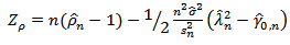 | (5) |
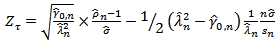 | (6) |
 when j=0, then
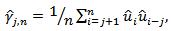
  is a maximum likelihood estimate of the variance of the error terms, whiles for
  is an estimate of the covariance between two residual terms j periods apart.
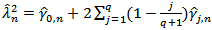 , if there is no autocorrelation between the residual terms,
  for
for then
then  . Replacing,
  in
in  , it reduces to;
 , which is a t-statistic in the standard Dickey-Fuller (DF) equation. Hence if there is no autocorrelation between the error terms, then the PP test is equal to the DF statistic with constant and time trend.Also, when the covariance are equal, then
  , thus the error terms have constant variance property (Homoscedastic), and
  which is the same as the DF test.
  is an ordinary least square (OLS) unbiased estimator of the variance of the residual error terms, where
  is the OLS residual, k is the number of covariates in the regression, q is the number of Newey-West lags to use in the calculation of
  is the parameter estimate of the PP regression model and
  is the OLS standard error of
  . The ADF and PP test discussed above have a weakness of not detecting the presence of structural breaks in the time series. If the structural changes are not allowed for in the specification of an economic model, but are present, the results may be bias towards the erroneous non-rejection of the non-stationarity hypothesis ([13]; [14]). Zivot and Andrews [12] therefore proposed a test procedure for unit roots that detect a single-term structural break point endogenously in the data such that the bias in the usual unit root test such as ADF and PP test can be reduced. This study used the proposed ZA test to check whether or not the rates studied were covariance stationary in the presence of any structural changes. The model endogenises one structural break in the series;
 | (7) |
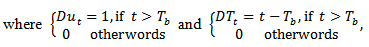
as  | (8) |
 is the time of break,
  is a sustained dummy variable capturing a shift in the intercept and
  represents another dummy variable representing a break in the trend occurring at time
  .
. 
 is chosen to minimized the one-sided t-statistic of
  in equation (7) and (8). Thus a break point is selected where the t-statistic from the ADF test of unit roots is minimal.
2.2. Vector Autoregressive (VAR) Modeling
A VAR (p) process consists of a set of k endogenous variables  and is given by;
 | (9) |
where 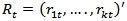 is a
is a  random vector of the rates,
 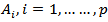 is fixed
  coefficient matrices,
 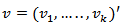 is a fixed
  vector of intercept and
 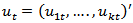 is a
is a  white noise series. Given sufficient starting values, a VAR process generates stationary time series with time invariant means, variances and covariance structure. This stability is determined by evaluating the reverse characteristic polynomial;
 | (10) |
A VAR (p) process is stable if the reverse characteristic polynomial has no root in and on the complex unit circle (thus the process is stable if  [15]). If the VAR (1) model is not stable, then either some, or all of the variables in the VAR (p) process are integrated of order one (I(1)). In practice, the VAR (p) is stable if the eigenvalues of the parameter matrix,
  are less than one in modulus
  . The stationarity of the VAR/VEC (p) model enables us to write the VAR (p) process as an invertible moving average process from which further inference such as Impulse Response Analysis can be made.
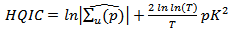
2.3. VAR Lag Order Selection
This study used the Akaike Information Criterion (AIC) [16], Schwarz Bayesian Information Criterion (SBIC) [17], and Hannan-Quinn Information Criterion (HQIC) [18], to determine the optimal lag order of the VAR (p) process of the set of rates. These criteria are given by;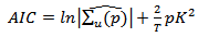 | (11) |
 | (12) |
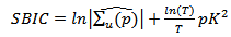 | (13) |
where  denotes the number of observations in the data,
  assigns the lag order,
 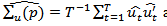 and K is the number of parameters in the statistical model. For all the criteria,
  is chosen so that the value of the criterion is minimized.
2.4. Model Diagnostics Test
This study employed the univariate Ljung-Box test and ARCH-LM test to test whether or not the residuals of the individual equations of the VAR (p) process are free from serial correlation and conditional heteroscedasticity respectively. The study also used multivariate Ljung-Box and multivariate ARCH-LM tests to check for the presence or absence of serial correlation and conditional heteroscedasticity in the residuals of the overall VAR(p) model estimated. The Cumulative Sum (CUSUM) test model diagnostics was also used to further check for stability of the parameters of the VAR model fitted.
2.5. Granger Causality Test
The idea behind Granger causality is that, if a variable  affects z , then
  should improve the prediction of variable z. A stationary variable
  is Granger causal for another stationary variable
  , if past values of
  has additional power in predicting
  after controlling for past values of
  [19]. If a stationary variable improves the prediction of another stationary variable, then the error of forecast of the latter becomes minimal. Causality can be unidirectional, bilateral or independent [20].
2.6. Impulse Response Function (IRF) Analysis
The impulse response analysis was used to examine the dynamic interactions between the endogenous variables over time. IRF enables us to determine the response of one variable to an impulse in another variable in the system, which involves a number of further variables as well. It is based on the Wold representation [15] of the moving average model of a VAR (p) process. This Wold representation based on orthogonal errors  is given by;
 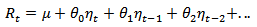 | (14) |
where  is a lower triangular matrix. The impulse responses to the orthogonal shocks
  are
are 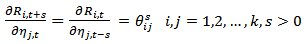 | (15) |
where  is the
  element of
  . For
. For variables there are
  possible impulse response functions.
2.7. Forecast Error Variance Decomposition (FEVD)
The FEVD was used to determine the contribution of the  variable to the h-step forecast error variance of the
  variable. If the
  variable shocks explain none of the forecast error variance of the
  variable at all forecast horizons, then the
  sequence is exogenous. Also, if the
  variable shocks explain all the forecast error variance in the
  sequence at all forecast horizons, then the
  variable is entirely endogenous. The FEVD is given as;
 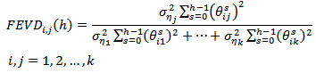 | (16) |
where  is the variance of
  . A VAR (p) process with
  variables will have
  values.
2.8. Chi-square Goodness of Fit Test
The Chi-square goodness of fit test is a statistical technique for comparing observed data with expected or predicted data according to a specified hypothesis. The VAR (p) model fitted was cross validated by an out-sample forecast from January, 2012 to October, 2012. The chi-square was used in this research to test whether or not there exist a significant difference between the observed sample rates and the out-sample forecasted rates of the VAR model. The chi-square statistic is given as;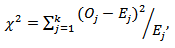 | (17) |
with k-1 degrees of freedom. Where  is the observed rate and
  is the expected rate and k is the number of rows in the forecasted data (sample size).
3. Results and Discussion
3.1. Fitting the VAR Model
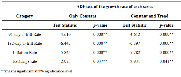
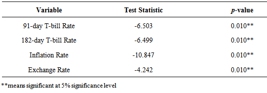
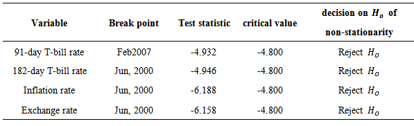
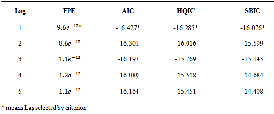
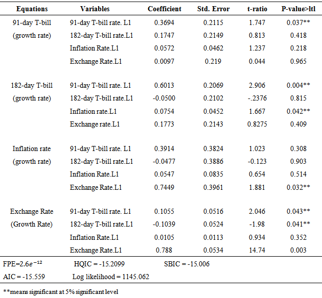
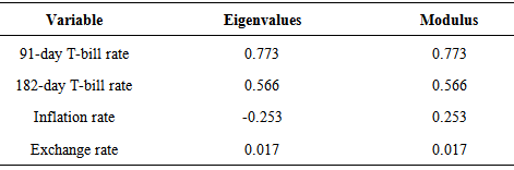
The stationarity of the variables studied were investigated; Graphical time series plots of the four rates as shown in Figure 1, indicates that each growth rate series fluctuates with constant variation about a fixed point and thus gives an indication of covariance stationarity. The Augmented Dickey-Fuller test performed on the individual growth rates series, with constant only and with constant and time trend shown in Table 1, revealed that the growth rates of each series were indeed covariance stationary. This was justified by a significant ADF test statistic at the 5% significance level. A significant PP test statistic of each series was also obtained at the 5% significance level as shown in Table 2, thus showing that the growth rate series of the four variables are covariance stationary. Additionally, the ZA test which test for unit roots in the presence of structural breaks in a series further affirms that the growth rates of each series were covariance stationary in the presence of structural breaks as shown in Table 3. This confirms that, the growth rates of each of the variables do not contain unit roots, hence are stationary processes.The optimal maximum lag order, p for the VAR process was assessed using four lag order selection criteria. As shown in Table 4, the AIC, HQIC, SBIC and Finite Prediction Error (FPE) all selected lag one (1) as the optimum lag order for the VAR process; since lag order one (1) had the least AIC, SBIC, HQIC and FPC values. Thus a four dimensional VAR (1) model was fitted to describe the relationship between these rates over time.As shown in Table 5, each endogenous variable is fitted on its own lag 1 value and the lag 1 values of the other endogenous variables. The results revealed that, the lag 1 value of the growth rate of the 182-day T-bill, Inflation rate and Exchange rate are not statistically significant at 5% significance level in predicting the growth rates of the 91-day T-bill rate whiles the lag 1 value of the 91-day T-bill is a useful predictor of itself at the 5% significance level. Also, the lag 1 estimate of the growth rate of the 91-day T-bill rate and Inflation are statistically useful in predicting the growth rate of the 182-day T-bill rate since they are statistically significant at the 5% significance level whiles the lag 1 values of the 182-day T-bill rate and Exchange rate are not useful predictors of the growth rate of 182-day T-bill. Only the lag 1 value of exchange rate is useful in predicting the growth rates in Inflation rate whiles the lag 1 values of the 91-day T-bill, 182-day T-bill and inflation rates are not useful predictors. Also, lag 1 values of the growth rates of the two T-bill rates and lag one (1) value of exchange rate are statistically useful in predicting the growth rates in exchange rates whiles Inflation rate does not.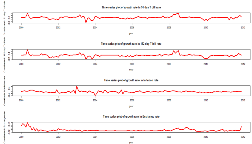 | Figure 1. Time series plots of growth rate of the rates |
Table 1. ADF Test of the Growth Rates of each Series
 |
| |
|
Table 2. PP Test of the Growth Rates of each Series
 |
| |
|
Table 3. ZA Test of Growth Rates of each Series
 |
| |
|
Table 4. Lag Order Selection for Fitting VAR Model
 |
| |
|
Table 5. VAR (1) Model for the Four Rates
 |
| |
|
Statistical Inference on the variables studied using the VAR (1) model depends crucially on the stability of the model parameters over time. The stability of the VAR (1) model was therefore investigated as shown in Table 6. The results revealed that, the model parameters were structurally stable over time; since all the eigenvalues of the parameters matrix have modulus less than one (1). This affirms that all the growth rates used in fitting the VAR (p) process was covariance stationary, as revealed by the ADF, PP and ZA tests thus affirming that the VAR (1) model fitted is a stable process. The VAR (1), without intercept, is given by  and estimated as;
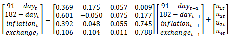 for
for 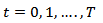
Table 6. VAR (1) Stability Condition
 |
| |
|
3.2. VAR (1) Model Diagnostics
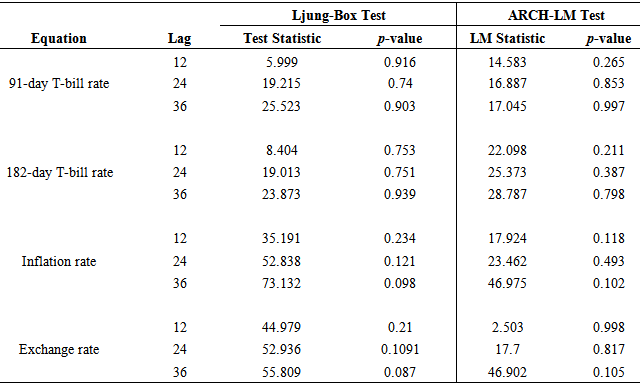
To ensure that the fitted VAR (1) model is adequate, both univariate and multivariate model diagnostic tests were performed. The univariate model diagnostic test, checked whether the residuals of the individual models in the VAR (1) model were white noise series whiles the multivariate model diagnostics checked whether the residuals of the overall VAR (1) model were white noise series. The univariate Ljung-Box test and ARCH-LM tests as shown in Table 7, showed that the residuals of the four individual models were free from serial correlation and conditional heteroscedasticity at lags 12, 24 and 36 since the p-values of the chi-square statistic exceeds the 5% significance level at all these lags. This shows that, the residuals of the four individual models are uncorrelated, have zero mean and have a constant variance over time; therefore they are white noise series. In addition, from the diagnostics plots of the standardized residuals for each model as in Figure 2, it is seen that, the residuals are random with constant variation around the zero line; hence give an indication that they have a constant variance and zero mean. These together show that the residuals of the 91-day T-bill rate, 182-day T-bill rate, Inflation rate and Exchange rate equations are white noise series. | Figure 2. Residual plots of the individual VAR equations |
Table 7. Univariate Ljung-Box Test and ARCH-LM Test of VAR (1) model
 |
| |
|
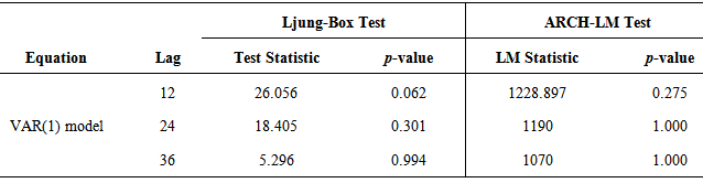
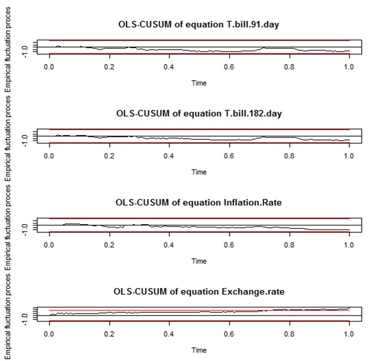
The adequacy of the overall VAR (1) model was investigated by the multivariate Ljung-Box and ARCH-LM test as shown in Table 8. An insignificant Ljung-Box statistic and ARCH-LM statistic were obtained at 5% significance level, indicating that the residuals of the VAR (1) processes are free from serial correlation and conditional heteroscedasticity; hence are white noise series. The VAR (1) model was further tested for stability using the CUSUM test. As seen from the CUSUM plot of each model in Figure 3, the cumulative residuals of each model fall within its 95% confidence limit indicating that, their individual mean are not significantly different from zero and have a constant variance. This further shows that the parameters of each model were structurally stable over time.Table 8. Multivariate Ljung-Box and ARCH-LM test of VAR (1) model
 |
| |
|
 | Figure 3. CUSUM plots of the Rates |
3.3. Granger Causality with VAR (1) Model
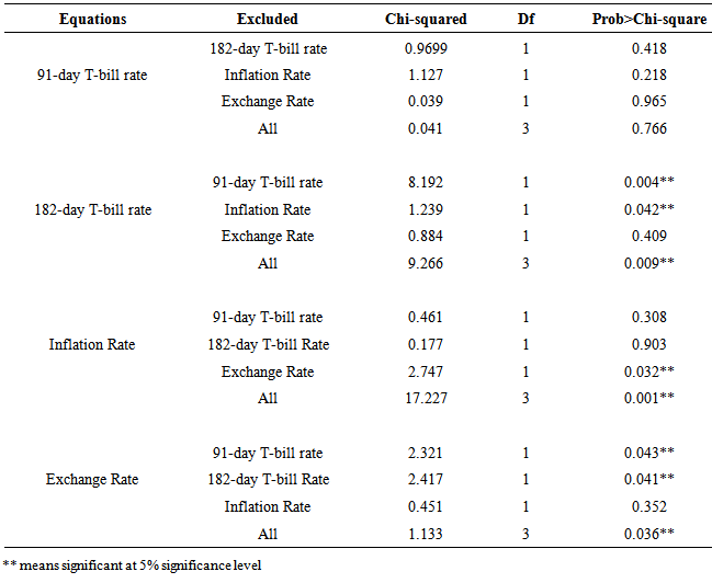
The VAR (1) model was used to investigate Granger causality among the set of rates studied to determine which growth rates have additional power in improving the prediction of growth rates of the other rates over time. The results, shown in Table 9, revealed that the 182-day T-bill rate, inflation rate and Exchange rate, individually and their linear combination does not Granger-cause the 91-day T-bill rate. This is seen from an insignificant chi-square statistic obtained for these individual rates and their combination at the 5% significance level. This implies that, there is no relationship between the 91-day T-bill rate and these variables; thus growth rates in these variables cannot improve prediction of the growth rate in the 91-day T-bill rate. Table 9. Granger Causality Test
 |
| |
|
The results also showed that, the 91-day T-bill rate Granger-cause the 182-day T-bill rate indicating that there is a unidirectional causality between the 91-day T-bill rate and the 182-day T-bill interest rate. This in addition indicates that, growth rates in the 91-day T-bill rate can improve the prediction of the growth rates of the 182-day T-bill rate whiles growth rates of the 182-day T-bills rates cannot significantly improve the prediction of the 91-day T-bill rate. Also, inflation rate Granger-cause the 182-day T-bill rate whiles the 182-day T-bill rate does not Granger-cause inflation rate, which also indicate a unidirectional causality between the 182-day T-bill and inflation rate. The exchange rate alone does not Granger-cause the 182-day T-bill rate whiles the 182-day T-bill alone Granger-causes the exchange rate indicating a unidirectional causality between exchange rate and the 182-day T-bill rate. This implies, pasts growth rates of the 182-day T-bill rates can improve the prediction of future growth rates of exchange rate but past growth rates of exchange rate alone cannot improve prediction of growth rates in the 182-day T-bill rate. However, a linear combination of the 91-day T-bill rate, Inflation rate and exchange rate together Granger-causes the 182-day T-bill rate. Additionally, growth rates in exchange rate Granger-cause growth rates in the Inflation rate whiles inflation rate does not Granger-cause the growth rates of exchange rate. The growth rates in the 91-day and 182-day T-bill rates individual do not Granger-cause inflation rate but when combined with exchange rate, they Granger-cause Inflation. This implies that, the growth rates in the two T-bill rates individually cannot improve the prediction of the growth rates in the inflation rate but that of exchange rate can.Lastly, the 91-day T-bill rate and 182-day T-bill individually Granger-cause the exchange rate, which indicates that the growth rates of the 91-day T-bill and 182-day T-bill rates individually can improve the prediction of the growth rates in exchange rate after accounting for past values of exchange rate itself. However, inflation rate does not Granger-cause exchange rateunless combined with other factors.
3.4. Impulse Response Function (IRF) Analysis with VAR (1) Model
The impulse response functions as shown in Figure 4 depicts the way the rates in the model interact following a shock in the VAR (1) model. When the impulse variable was the 91-day T-bill rate, in the first period, the 91-day T-bill rate showed a positive reaction to a shock in its own values followed with a continues negative reaction up to period eight and a stable response for the rest of the periods. The 182-day T-bill rate reacted positively to a shock in the 91-day T-bills rate in the second period followed with a negative response from the third to the sixth period and then a stable response for the rest of the periods. Inflation rate also reacts positively at period two to a shock in the 91-day T-bill, followed with a sharp negative reaction up to period six and a stable response thereafter. Exchange rate reacted positively to a shock in the 91-day T-bill rate for the first, second and third periods followed with a stable response in period four and finally a negative response for the rest of the periods.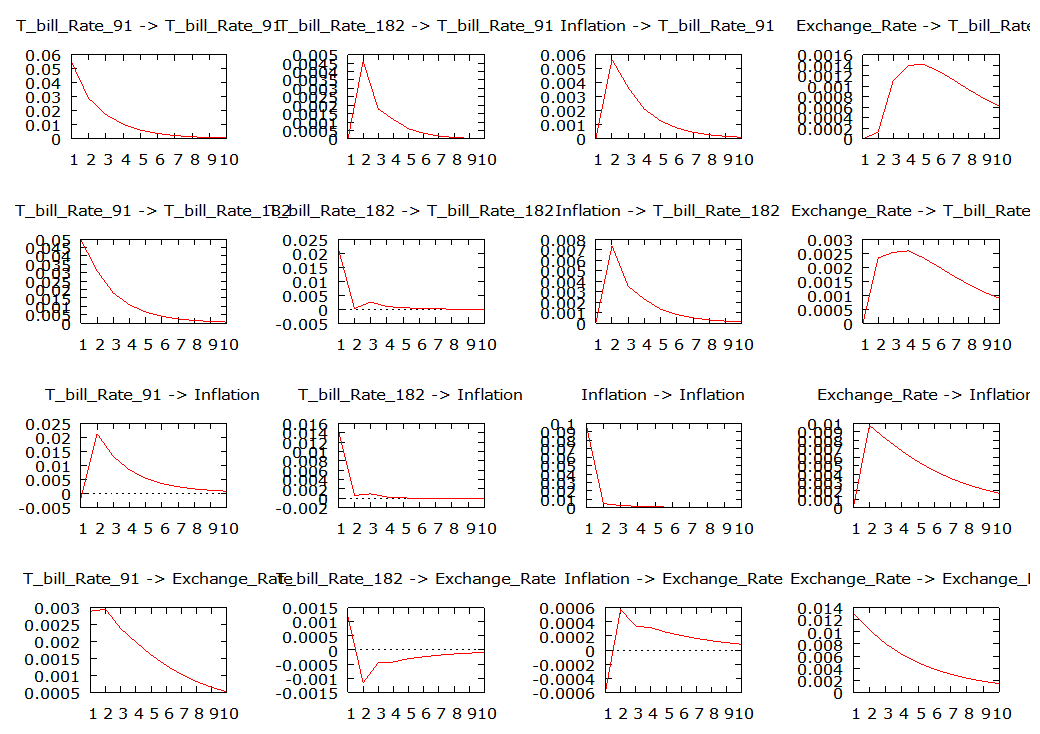 | Figure 4. Impulse Response Plots of the Relationship between the Rates |
When the impulse variable was the 182-day T-bill rate, the 91-day T-bill rate showed a positive reaction to a shock in the 182-day T-bill rate in the first period which was followed with continues negative response up to the last period. In the first and third periods, the 182-day T-bill rate showed a positive response to a shock in its own values, the second period showed a negative response and then a stable response to its own shocks onwards. Inflation rate showed a positive reaction at the second period, negative between the third and sixth periods and a stable response to a shock in the 182-day T-bill rate for the rest of the periods. Exchange rate reacted positively at the second period to a shock in the 182-day T-bill rate. The third and fourth period showed a stable response to a shock followed with a negative response afterwards.When the response was inflation rate, the 91-day T-bill rate reacts positively at the second period, followed by a negative reaction up to the seventh period and a stable reaction for the rest of the periods. The 182-day T-bill showed a positive reaction in the first period, a negative response at the second period with a stable response for the rest of the periods. The inflation rate itself reacts positively at the first period to a shock in its own values, a negative reaction at the second period and a stable response for the rest of the periods. Exchange rate reacts positively at the second period to a shock in the rate of inflation and a sharp negative reaction for the rest of the periods. For exchange rate as the impulse variable, the 91-day T-bill reacts positively at the first period to a shock in the exchange rate, a stable response at the second period followed with a negative linear response for the rest of the periods. The 182-day T-bill rate reacted positively at the first and third periods, negatively at the second period and stabilized after the third period. Inflation rate reacts negatively at the first and third periods with a slow negative response for the rest of the periods. Exchange rate showed a positive reaction at the first period to its own shock, followed with a continuous negative response for the rest of the periods.
3.5. Forecast Error Variance Decomposition (FEVD) with VAR (1) Model
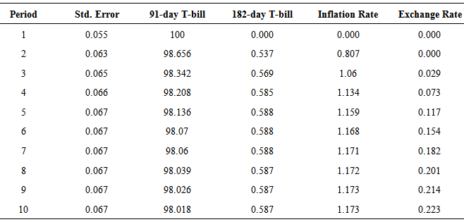
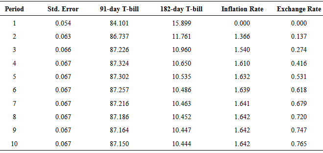
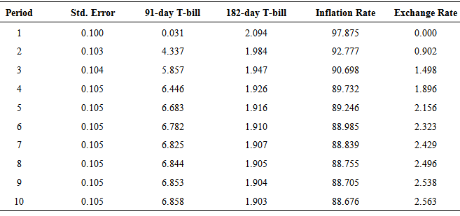
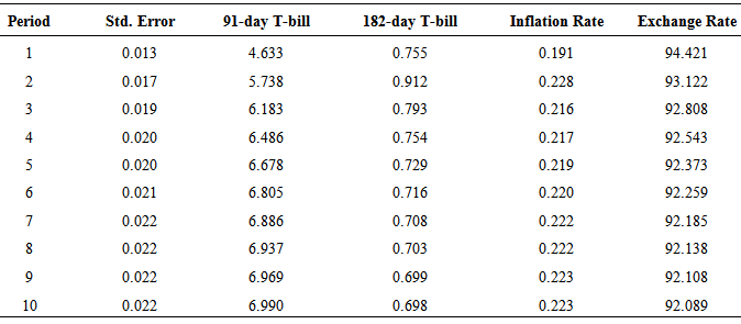
The variance decomposition was used to determine the proportion of forecast error variance of each rate that was explained by itself and by the other endogenous rates in the study. Table 10 gives the variance error decomposition of the 91-day T-bill rate. It was realized that, much of the forecast error variance in the 91-day T-bill rate have been explained by innovations in the 91-day T-bill rate itself. For instance, in the tenth period, about 98.02% of the error variance in the 91-day T-bill is explained by innovations in the 91-day T-bill rate, whiles only about 0.59%, 1.17% and 0.22% of its error variance is explained by the 182-day T-bill rate, Inflation and Exchange rate respectively. This then supports results by the VAR (1) model and Granger causality that, the 182-day T-bill rate, Inflation rate and Exchange rate do not contribute significantly to the prediction of the 91-day T-bill rate.From the forecast error variance decomposition of the 182-day T-bill rate shown in Table 11, the influence of the 91-day T-bill rate contributes the most in forecasting the uncertainty of the 182-day T-bill rate. At period ten, about 87.15% of the error variance in the 182-day T-bill rate have been explained by innovations in the 91-day T-bill, whiles about 10.44% of the variance is explained by innovations in the 182-day T-bill itself, 1.64% explained by innovation in inflation rate and 0.76% by the exchange rate. The results of 182-day T-bill variance decomposition also agrees with views of the Granger causality test and the estimated VAR (1) model which revealed that, past growth rates of the 91-day T-bill rate is the most influencing determinant of the growth rates of the 182-day T-bill rate. It also confirms the unidirectional relationship between the 91-day T-bill and the 182-day T-bill rate. Apart from inflation itself, the 91-day T-bill rate is the most influential variable in forecasting the uncertainties of inflation as seen in Table 12. For instance, at period ten about 88.68% of the error variance in inflation is explained by innovations in the inflation rate itself, 6.86% explained by innovations in the 91-day T-bill rate, 1.90% by innovations in the 182-day T-bill rate and 2.56% by the exchange rate. Lastly, apart from exchange rate, which explains about 92.09% of the error variance in itself, the 91-day T-bill rate contributes most in forecasting the uncertainty of the exchange rate as seen in Table 13. At period ten, 6.99% of the error variance in the exchange rate is explained by innovations in the 91-day T-bill rate, 0.70% by the 182-day T-bill rate and 0.22% explained by inflation rate.
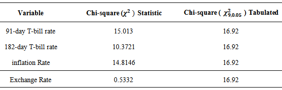
3.6. Chi-Square Goodness of Fit Test for VAR (1) Model
The VAR (1) model fitted was cross validated with an out-sample forecast from January, 2012 to October, 2012. The forecasted growth rates were then compared with the actual growth rate within the period using the chi-square goodness of fit statistic. The Chi-square test results as shown in Tables 14 showed that, there is no significant difference between the observed growth rates and the forecasted growth rates for all the variables as shown by an insignificant chi-square statistic of 15.013 for the 91-day T-bill rate, 10.3721 for the 182-day T-bill rate, 14.8146 for inflation and 0.5432 for exchange rates which are all less than the Chi-square test statistics value of 16.9200. This shows that the fitted model produce values that mimic the behavior of the rates over time, although the values of the observed and expected are not exactly the same. Table 10. Forecast Error Variance Decomposition for 91-day T-bill rate
 |
| |
|
Table 11. Forecast Error Variance Decomposition for 182-day T-bill rate
 |
| |
|
Table 12. Forecast Error Variance Decomposition for Inflation rate
 |
| |
|
Table 13. Forecast Error Variance Decomposition for Exchange rate
 |
| |
|
Table 14. Chi-square Goodness of Fit Test
 |
| |
|
4. Conclusions
In this research, the relationship between Treasury bills, inflation and exchange rates in Ghana was investigated. The VAR (1) model, Granger-causality and FEVD showed that, growth rates of the 91-day T-bills depends on its own past values but independent of inflation, 182-day T-bill and exchange rates. Growth rates of the 182-day T-bill rate depends greatly on past growth rates of the 91-day T-bill but independent of itself, inflation and exchange rates. Future occurrences of growth of inflation also depend only on exchange rates behavior and growth rates of the exchange rate depends on the two T-bill rates and on its own past occurrences. The results also showed that, past values of inflation rate were positively correlated with past values of the two T-bill rates; indicating that a continuous increase in inflation results in a continuous increase in these T-bill rates although the effects is weaker. Therefore, a continuous depreciation of the Ghana cedi leads to high and more volatile inflation which leads to increases in interest rates. It is therefore recommended that, the government should pay much attention to both exchange rate and inflation dynamics over time due to their relationship with interest rates. The government should also ensure that, inflation rates are kept low to keep the levels of interest rate stable over a period of time. Although interest rate seems to be increasing with increasing inflation, a continuous increase in inflation can also lead to high prices of commodities and services in the country and this can make the returns of investments not worth enough; investors are therefore advised to consider factors such as inflation and the value of the local currency and its performance in the financial market in their investment decisions, so that best decisions can be made if investments in securities at a particular time is worthwhile. Also, both univariate and multivariate ARCH-LM test and Ljung-Box test showed that the residuals of the model are white noise series.
References
| [1] | Ado A., (2013). The Impact of Treasury Bill Rate and Interest Rate on the Stock Market Returns: Case of Ghana Stock Exchange. www.acedmia.edu.com. Assessed on 6th January, 2014. |
| [2] | Wikipedia, (2013). Economic Stability.en.wikipedia.org/wiki/Economic-Stability. Assessed on 1st April, 2014. |
| [3] | Wise GEEK, (2014). What is economic stability? www.wisegeek.org/what is economic stability.htm. Assessed on 1st April, 2014. |
| [4] | Engle, R. F., and Granger, C. W. J., (1987). Cointegration and error correction: Representation, Estimation and Testing. Econometrica.55:251-276. |
| [5] | Nguyen, T. and Seiichi, F., (2007). Impact of the Real Exchange Rate on Output and Inflation in Vietnam: A VAR approach. Discussion Paper No.0625. |
| [6] | Noer, A. A., Arie J. F., and A. Piter., (2010). The relationship between inflation and real exchange rate, comparative study between Asian+3, the EU and North America. European Journal of Economics, Finance and Administrative Sciences ISSN, Issue 18: 1450-2887. |
| [7] | Goldfajn, I., and Gupta, P., (1999). Does Monetary Policy Stabilize the Exchange Rate Following a Currency Crisis? International Monetary Fund Working Paper, WP/99/42, Washington D. C. |
| [8] | Berument, H., (1999). The Impact of Inflation Uncertainty on Interest Rates in the UK. Scottish Journal of Political Economy,46(20): 207-218. |
| [9] | Luguterah A. and Logubayom I. A., (2014). Modelling Relationships between Treasury Bills, Inflation and Exchange Rates in Ghana: A Co-integration Approach. Journal of Statistical and Econometric Methods, 3(2): 75-92. |
| [10] | Dickey, D. A., and Fuller, W. A. (1979). Distribution of the Estimators for Autoregressive Time Series with a Unit-root. Journal of American Statistical Association, 74: 427-431. |
| [11] | Phillips, P. C. B., and Perron, P., (1988). Testing for a unit root in time series regression.Biometrika75: 335–346. |
| [12] | Zivot, E., and Andrews, K., (1992). Further Evidence on the Great Crash, the Oil Price Shock, and the Unit Root Hypothesis. Journal of Business and Economic Statistics, 10 (10): 251-70. |
| [13] | Perron, P., (1989). The Great Crash, the Oil Price Shock, and the Unit Root Hypothesis. Econometrica, 57: 1361-1401. |
| [14] | Perron, P., (1997). Further Evidence on Breaking Trend Functions in Macroeconomic Variables. Journal of Econometrics, 80 (2): 355-385. |
| [15] | Lutkepohl, H., (2005). New Introduction to Multiple Time Series Analysis. Springer. |
| [16] | Akaike, H. (1974). A new look at the Statistical Model Identification. IEEE Translation on Automatic Control, AC-19:716-723. |
| [17] | Schwarz G. E., (1978). Estimating the Dimension of a Model. Annals of Statistics, 6:461-464. |
| [18] | Hannan, E. and Quinn, B., (1979). The Determination of the Order of an Autoregression. J. Roy. Statist. Soc. Ser. B 41: 190–195. |
| [19] | Gelper, S., and Croux, C. (2007). Multivariate Out-of-Sample Tests for Granger causality. Computational Statistics and Data Analysis.51: 3319-3329. |
| [20] | Gujurati, D. N., (2003). Basic Econometrics. Fourth Edition. New Delhi, the McGraw-Hill Co. |
 Abstract
 Reference
 Full-Text PDF
 Full-text HTML