1. Introduction

The word equilibrium is derived from the Latin word aequlibrium which means equal balance (Jhingan 2009 p74).

An equilibrium is a position from which there is no net tendency to move. We say net tendency to emphasize the fact that it is not necessarily a state of sudden inertia but may instead represent the cancellation of power (Stigler 1966).

Equilibrium denotes in economics absence of change in movement (Mehta 2003). In other words, it is a market situation where all decisions by the participants are in uniticity with each other. A market or an economy or any other group of persons or firms is in equilibrium when none of its members feels impelled to change his behavior (Scitovsky 1951).

For a group to be in equilibrium therefore all its members must be in equilibrium and the equilibrium behavior of each member must be compatible with the equilibrium behavior of all its members. In economics, equilibrium implies a position of rest characterized by absence of change. It is a state where there is complete agreement of the economic plans of the various market participants so that no one has a tendency to revise or alter this decision (Jhingan 2009 p74). Some of the notable contributions to the theory of equilibrium are General equilibrium by Leone Walras in his pioneering work Elements of pure economics (1977). General equilibrium theory both studies economies using the model of equilibrium pricing and seeks to determine in which circumstances the assumptions of general equilibrium will hold. Partial equilibrium on the other hand is a condition of economic equilibrium which takes into consideration only a part of the market, ceteris paribus, to attain equilibrium. As defined by George Stigler, "A partial equilibrium is one which is based on only a restricted range of data, a standard example is price of a single product, the prices of all other products being held fixed during the analysis (Jain 2007).

In game theory, the Nash equilibrium is a solution concept of a non-cooperative game involving two or more players, in which each player is assumed to know the equilibrium strategies of the other players, and no player has anything to gain by changing only their own strategy ( Osborne, Martin J, and Rubinstein 1994). Nash equilibrium has been used to analyze hostile situations like war and arms races (Schelling Thomas 1960). As good as these contributions and many lot more are, they only shed little light to address the issue of changes in the level of interaction between demand and supply in the course of time.

2. Statement of the Problem

Equilibrium is a balanced region where a single activity of interaction and intersection takes place by the forces of demand and supply that are influenced by other factors.

Over the years the various scholarly contribution to the concept of equilibrium has centered around the interaction between demand and supply and its long and short run relationship with price, market conditions such as perfect and imperfect markets and others, and forces that make up and influence equilibrium with little or no highlight on the issue of a favorable and unfavorable balance of equilibrium. The interaction of demand and supply, its impact on price increase or decrease in the short and long run and incentives to increase output which later results to equilibrium in the long run in markets such as perfect competition, imperfect competition, monopolistic competition and the rest etc. the tendency for producing firms to make high profit in the short run and later low profit later in the long run which end up discouraging intending firms to enter into the market because of fallen price in the long run, which inevitably leads to equilibrium have been the basic interpretation of equilibrium.

In this study however we will be looking at the equation Qs=Qd and its implications to firms and the economy, its favorability and unfavorability. It is on this note that this study seeks to address the following questions.

Firstly what are the issues surrounding the equation Qs=Qd? Secondly what is the favorable and unfavorable balance of the equation Qs=Qd? Thirdly what are its implication to firms and the economy? Fifthly what is the relationship between time and equilibrium? What are the other set of properties of Qs=Qd apart from the ones proposed by Huw Dixon 1990?

3. Significance of Study

This study reveals the relationship between time and equilibrium. Secondly it reveals new sets of properties of the equation Qs=Qd besides the ones proposed by Huw Dixon 1990. Thirdly it reveals the implication of the rate of interaction between demand and supply to firms. Fourthly this study reveals that equilibrium is established at all levels of demand and supply interaction which brings about the equation Qs=Qd but which varies in the chain of time that ultimately leads to zero equilibrium. This study also reveals the concept of zero equilibrium.

To begin with, the equation Qs=Qd shows the positions of firms which determines level of revenue or loss for firms and the economy. When firms cover there costs a favorable balance of Qs=Qd occurs that is, Qs=Qd⁺¹. The +1 is the profit that was made that covered cost.

4. Favorability and Unfavorability of Qs=Qd

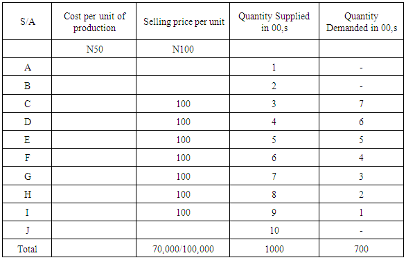
Equilibrium is either favorable or unfavorable when its balance favors firm or not.

Table 1 shows a favorable balance of equilibrium because out of the 1000 quantity supply of cars 70% were sold. And revenue of 70,000 was made. It means cost has been covered. This is because out of Total cost of 50x1000=50,000 (cost per unit x total unit) of producing the 1000 cars, revenue of 70,000 was made. This can be calculated as Total cost of production minus Sales (50,000-70,000 = 20,000). This shows that there is a favorable balance of the equation Qs=Qd⁺¹

An unfavorable equilibrium balance rarely occurs but can occur in times of economic cycles were firms are not able to sell there products above the average cost. An instance was during the economic melt down where firms folded up because they couldn’t cover there costs of production. To illustrate this phenomenon we study firms under business cycles or economic crisis which many times lead to firm fold up.

Table 1. Showing a favorable balance of equilibrium

The table 2 shows an unfavorable balance of equilibrium.

In the table 2 we see that during the business cycle or economic melt down firms were not able to generate good demand which made there prices fall below the average cost. An extreme form of this scenario is when firms do not at all generate demand for there products which will automatically lead to firm fold up.

We can mathematically illustrate the table as Qs=Qd^-1.

Table 2. Showing an unfavorable balance of equilibrium

In tables 1 and 2, the concentration is no longer at point E but from point A to J. In table 3 the concentration is no longer at period 4 but from period 1-5.

5. Relationship between Time and Equilibrium

Equilibrium is determined by time. The level of interaction between demand and supply changes with time. Qs=Qd varies from time to time. Thus equilibrium is established by the interaction of demand and supply with price as the referee but this interaction level changes from time to time till at the point where Qs=Qd is exhausted. We can understand this phenomenon by looking at diminishing marginal utility For instance a consumer buys iPhone 4S. He will be very excited at the moment but the level of this excitement varies from time to time till it reaches a point where there is no longer excitement and he decides to sell the phone. A car that was produced ten years ago is no longer in the market. This is because there is no longer interaction between Qd and Qs which can be represented as Qs⁰=Qd⁰ this equation is also called zero equilibrium.

If in the current period or short-run firm sells only Nth% of it’s output, it means supply Nth% generated demand of Nth%. Thus supply Nth% generated demand Nth% therefore Nth%Qs=Nth%Qd which is supported by Says law of markets that supply creates demand. Thus we try to prove that equilibrium is not only achieved in the long-run but that equilibrium is already established when supply generates demand at the current periods. Therefore equilibrium is a balance. Thus when forces interact there is a balance that varies with each stage of interaction, therefore if out of 1000 cars Nth% were sold out it means Nth% of supply of output generated Nth% of demand which the theory represents as Nth%Qs=Nth%Qd, the difference is that the level of interaction between Qs and Qd changes or varies with time. This view is applied in this instance to single products and not total products or total industrial output.

For instance Micro-Soft produces Windows XP in the current period; we assume 100million windows XPs for sale. This theory proves that for all levels of interaction of demand and supply equilibrium is established. For illustrative purpose we divide periods into three.

In period 1 If out of the 100million Windows XP that micro-soft produce it sells only 30%, this theory emphasizes that the 30%Qs generated 30%Qd or 30%Qs=30%Qd. In period 2 this level of interaction will change either increase or decrease. In period 3 it will either change or remain as before either with the same prices or with different prices.

This theory sees the interaction of demand and supply as equilibrium in itself whether in the long or short-run because the difference between long or short-run is the level of interaction between demand and supply. While a consumer buys a new product and is excited with it, his interest and excitement of the product fades away with time or in the long run, in other words his interest has reduced or rate of his excitement has reduced in the long run which will totally fade or becomes zero with time. That means his level of interest changes or varies in the chain of time so also is equilibrium.

A change in the level of interaction between demand and supply varies in short and long run and will eventually become zero or what is called zero equilibrium. Therefore equilibrium as emphasized by this theory is the interaction of demand and supply but views a favorable interaction between these two when one is higher (which is to be to the firms’ advantage). Equilibrium is a varied level of interaction between Demand and Supply in the chain of time which will eventually become zero. For instance some goods produced by Sony or its fellows in the past ten years are no longer in production. Why? Because the level of demand and supply has reached a zero point but before this point the level of interaction deferred in the chain of time that is interest/demand kept decreasing till it reached zero point and thus Sony no longer produced the good again because there is no longer demand for the good.

6. What are the Implications of the Interactions between Rates of Demand and Supply?

Every production is aimed at covering cost. These covered costs are the revenue or expected revenue. Covering these costs involves the interaction of demand and supply. It can be viewed as Qs vs. Qd. Firms always make sure that Qs wins I.e by ensuring that Qs attracts more Qd. The implication of Qs losing is what makes firms to fold up especially during economic melt downs and business cycles. Firms go as far as employing various strategies to ensure that Qs wins. The picture here is that Qs=Qd⁺¹ it means cost has been covered and thus there is a favorable balance of equilibrium. This means that Qs attracted more Qd.

7. Properties of Qs=Qd

The properties of the above equation are

1. Revenue/ Loss

2. Interaction level

3. Percentage of sale

4. Market power or position.

5. Financial condition of firm

Points 3, 4 and 5 are determined by point 2. The rate of interaction between Qs and Qd brings about points 3, 4 and 5

Equilibrium is a three way relationship that varies in the chain of time. Let us assume a set of time periods {1, 2, 3… + N}. Between these periods the relationship between Price, Supply and Demand changes within these periods to the point where it becomes zero. I.e {1, 2, 3 …+ N} = 0. Once this relationship reaches zero, production of output ceases because Qs=Qd became zero I.e Qs⁰=Qd⁰.

This three way relationship in the chain of time works in the following Algorithm.

P= (supply and demand)

D= □ (price and supply)

S= □ (demand and price)

Price is determined by supply and demand. Demand also determines price and quantity supplied. Supply is equally determined by price and demand. Let’s look at the following points. High supply accompanied by low demand reduces price. High demand accompanied by low supply increases price. Low demand is tackled by decreasing price I.e. price manipulation determines demand and supply because high demand as a result of price reduction at an acceptable rate increases supply. These relationships vary in the chain of time which creates equilibrium.

Let us look at the tabular explanation of this phenomenon.

Table 3. Showing time variations or changes in equilibrium and the three way relationships of equilibrium

From the sets of periods {1, 2, 3, 4, and 5} we observe that price is determined by the interaction of demand and supply and supply is determined by price and demand is determined by influenced by price and supply. From the table we observe that the level of relationship between demand and supply and price changes in the chain of time or periods. The level of relationship between demand and supply varied from period to period. This implies that equilibrium is a function of time which is brought about by the relationship or interaction between demand, supply and price. This is because we can observe differences in the level of relationship from one period to another.

Thus the relationship Qs and Qd varies in the chain of time.

Assuming Average Cost is 50 and supply price is 75. The level of interaction between demand and supply in the chain of time will determine whether a firm will cover its cost at the supply price of 75.

If the interaction between demand and supply is high cost will be covered will be covered which will smoothen production in the next period. The coverage takes place at the chain of time. This creates the equation Qs=Qd⁺¹ or Qs=Qd^-1.

Assuming at the average cost of 50, a firm may set supply price at 75. The 25 price difference (75-50 I.e supply price less Average cost) is the expected level of revenue which is determined by the interaction of demand and supply. In the chain of time this interaction varies, thus the higher the interaction the more favorable equilibrium will be and the lower the interaction the more unfavorable equilibrium will be.

Let us look at this phenomenon

Total Output=1000 cars

Total Cost=50,000

Average Cost = 50

Supply price=75

Qd=700

Therefore a favorable balance of equilibrium occurs where

QdxQs at 75 SP= 700x75=52,500.

The high interaction of demand with supply generated a favorable equilibrium of 2500 I.e (Total Cost-Total revenue) 52500-50,000=2500. The 2500 is the ⁺¹ which is represented as Qs=Qd⁺¹. This indicates that cost of production of 50,000 has been covered and thus production in the next period will be in full capacity. But it is worth noting that this interaction was not achieved at the initial stage of supply. It only increased at the chain of time. This indicates that before Qd of 700 the interaction of demand and supply was low but kept increasing in the chain of time to 700. Thus this relationship will continue till at the stage where zero equilibrium Qs⁰=Qd⁰ is achieved i.e. there is no longer interaction between demand and supply. At this stage production of brand will cease to exist in the market.

These changes vary in the chain of time. Business cycles, economic meltdowns and other economic and financial factors may take place that will influence price to change either increase or decrease.

8. Conclusions

Qs=Qd is the heart beat of every transaction. For profit or revenue to take place it is hoped or expected that the interaction between these two forces becomes favorable which this paper mathematically represents as Qs=Qd⁺¹ which shows that cost has been covered or that Qs generated high Qd which covered cost thus making production in the next period in full capacity. When this happens we say there is a favorable balance of equilibrium. Favorable balance happens during normal business periods or periods outside business cycles or economic meltdowns or periods that do not make company prices to fall or demand fall.

ACKNOWLEDGEMENTS

Thanks to God Almighty for the inspiration to conduct this research.