Gang Liu
Technology Research Department, Macrofrontier, Elmhurst, New York
Correspondence to: Gang Liu , Technology Research Department, Macrofrontier, Elmhurst, New York.
| Email: |  |
Copyright © 2014 Scientific & Academic Publishing. All Rights Reserved.
Abstract
Supply function and Production Possibility Frontier (PPF) are basic concepts in Economics. We present a model that can give mathematic formula for PPF and the supply as a function of the price vector and capability parameters. With this Supply function, the generic Supply-Demand equilibrium problems can be solved numerically. We apply the supply-demand equilibrium to give optimal solutions for team work management problems or labor assignment problems. Concrete examples are given for managing an engineer team in Boeing Corporation.
Keywords:
Resource Allocation, Labor Assignment, Teamwork Management, Supply Function, Production Possibility Frontier, Supply-Demand equilibrium
Cite this paper: Gang Liu , A Mathematic Model for Supply-Demand Equilibrium and the Optimal Solution for Labor Assignment, American Journal of Economics, Vol. 4 No. 2, 2014, pp. 83-98. doi: 10.5923/j.economics.20140402.01.
1. Introduction
Production Possibility Frontier (PPF) is one of the basic concepts in Economics. PPF can be simply defined as the boundary of frontier of the economy’s production capabilities. Most of Economic books normally have a whole chapter to discuss PPF and its applications [1, 4, 10, 11]. Most of these text books discuss the PPF and supply function for two products and in qualitative format, as shown in Figure 1. It is well-known that the PPF is convex and the supply-price curve is an upward-sloping curve. However, no one has given the PPF nor supply function in mathematic formats. The law of supply and the law of supply-demand equilibrium are basic laws in modern economics. However, without knowing the supply function in mathematic format, these laws can be only discussed quantitatively, and the general supply-demand equilibrium cannot be solved numerically. In early 2002, we have given the PPF and supply function in mathematic format for any number of products [6]. In this paper, we first introduce the model that can formulate the PPF in mathematic format, and then derive the supply as a function of the prices of all products. Some of the basic economic theorems can be derived from the PPF formula, such as the convexity of the PPF curve, the Law of Supply, as well as supply elasticity. We also proposed methods for solving the general supply-demand equilibrium numerically. There are wide applications of the proposed PPF functions. As an example, we apply the PPF function and the Supply-Demand equilibrium equation to give optimal solution for team work management and labor assignment problems. Our analysis and test results show that the proposed model can improve production efficiency by 40% for most of the team work management problems.The rest of the paper is organized as follows. Section 2 introduces some useful notations and definitions. Section 3 formulates the PPF and the supply function for a micro system. Section 4 further formulates the PPF and the supply function for a macro system. Section 5 discusses the lower Production Possibility Frontier. Section 6 discusses the Law of Supply and the Elasticity of Supply. Section 7 introduces two methods for solving the supply-demand equilibrium. Section 8 introduces two special production possibility curves that can be used to show how efficiency of the PPF. Section 9 applies our supply function to a dummy system to show concrete PPF curves and supply curves. Section 10 discusses the best scenario and the worst scenario. Section 11 applies our model to solve the labor assignment problem for a labor oriented team. Section 12 shows a concrete example of labor assignment problem for project oriented team. In Section 13 and 14, we analyze the efficiency improvements by the optimal solution. Section 15 introduces two management methods that can reach the optimal solution for team work management. Conclusions are presented in Section 16.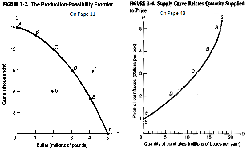 | Figure 1. This is a snapshot from Samuelson’s book “Economics” [11]. Without knowing the mathematic formats of the PPF and supply function, most of the Economics books can only discuss PPF, Supply, and supply-demand equilibrium quantitatively. We proposed a model that can give PPF and Supply as a mathematic function of the price as shown in Equation (17) |
2. Notations and Definitions
In order to describe our model and the PPF curve, let us first introduce some notations and definitions.
2.1. Notations
 : An economic system that contains some sub systems. It can be as small as a family, a firm, and can be as large as a country or the whole world.
  is also called a macro system compared with its sub systems.
 : An integer represents the total number of the sub systems in
  .
.  : An integer represents the total number of the products that are produced in
  .
.  : The ith unit or sub system in system
  . It could be an individual member, or a group of people, such as a firm or another economic system in
  . However, there are no overlaps between different Units. For example, if an individual has been included in one unit, the same individual can’t be included in another unit.
  is also called a micro system compared with its parent system.
 : The kth product that can be produced in system
  . Actually, the product here means any labor activities that can be done by any unit in
  . It can be a real product, a project, a job, a task, and anything that need to be done or produced by any unit in
  .
. : A time span that the above mentioned products are produced in
  .
. :
:  , which is the set of non-negative M-dimensional real vectors and with the original point
  excluded.
 : The same as
  . However, we use it to particularly represent the Production Space with its kth Cartesian coordinate representing the amount of a parameter related to
  product.
 : The demand amount of
  product that requested by
  .
.  : The maximum amount of
  product that can be produced by
  within time
  . Normally
  can be produced by
  when it uses all of its resources to work on product
  . All the
  make up an
  matrix, which is called the micro capability matrix of system
  .
.  : The amount of
  product that are actually produced by
  . All the
  make up a vector in
  , and is called micro supply vector.
 : The amount of
  product produced by the macro system
  . It is also called the macro supply of system
  . All the
  make up a vector in
  , and is called a macro supply vector of system
  .
. ;
;  : The price of the
  product in system
  .
.
2.2. Definitions
Definition: Micro System and Macro System: An economic system is called a macro system if it contains some sub-systems, such as the system  introduced above. An economic system is called a micro system if it is contained in a macro system, such as the sub-system
  described above. Definition: System Parameter: An economic parameter is called a system parameter if it is associated with an economic system. For example, the supply amount, demand amount, and price are all examples of system parameters. Definition: Micro Parameter and Macro Parameter: A system parameter is called a micro parameter if it is associated with a micro system, and is called a macro parameter if it is associated with a macro system. Some parameters may be associated with both micro system and macro system. As long as there is no confusion, we use the same alphabet character to represent a system parameter: if
  denotes a macro parameter associated with a macro system
  , then
  will be used to denote the same micro parameter associated with micro system
  .For example,
  and
and  represent the macro and micro supply amounts of product
  ,
,  and
and  denote the macro PPF of system
  and the micro PPF of the micro system
  correspondingly. Definition: Vector Parameter and Scalar Parameter: a system parameter may also be associated with each of the production, for example, supply amount normally means the amount of a product that can be provided by an economic system. In a system with
  products, a system parameter could be
  -dimensional with each component representing the amount associated with one product. These
  -dimensional parameters make up a vector in the production space
  , thus is called a Vector Parameter. A vector parameter can be represented by a vector in
  . Examples of vector parameters are: Supply, Demand, and Price. A system parameter is called a scalar parameter if it is one dimensional. Examples of scalar parameters are: income, GDP, revenue, etc.Additive Parameter: A system parameter is called additive parameter if the corresponding macro parameter can be derived by aggregating the same parameter over all of its micro systems. Or precisely, system parameter X is additive if
  | (1) |
Where  is a parameter reachable and meaningful to micro system
  , while
  is the same parameter reachable and meaningful to macro system
  .In our model, we tried to decompose the macro system
  into some micro systems
  , and divide the products into some products or tasks in such a way that some of the system parameters are additive, particularly, the supply amount, the demand amount, revenue, and income are all additive. However, the price parameter is not an additive parameter. Based on the above notations and definitions, we can say that the supply and demand are vector parameters and are additive, whereas the price is also a vector parameter, but not additive. The income, revenue, GDP, profit and loss are all additive scalar parameters. We are only interested in those parameters in this paper.
2.3. Known Parameters and Unknowns
Using the above notations, we can list the input data in table format. Basically, we assume the following data are known input data: , the production capability matrix for each micro system and for each product.
 : The macro demand of
  product that needs to be accomplished by system
  . We assume the following parameters are unknowns and need to be resolved: Price, micro supply, macro supply, micro income, macro revenue.
3. Micro PPF and Micro Supply Function of a Micro System
For any micro system  , let us assume that it can arrange its resources to make any requested products. However, its production amount for product
  should be limited to or bounded by
  due to its limited resources and capabilities. Any of its feasible production state will be a point or a vector in the production space
  . All of its feasible production vectors should be a bounded range in the production space
  . We call this bounded range as its micro Production Possibility Range (PPR) and denoted as
  . The upper boundary of
  is called the micro PPF, denoted as
  . Normally, as long as the micro system
  is small enough compared with macro system
  , each of the micro PPF can be approximated by the linear plane curve that passing the
  axis at
  in production space
  . Given the micro capability matrix, the micro PPF
  can be formulated as:
 | (2) |
 can also be expressed in the following format:
 | (3) |
Where  | (4) |
 is called the intrinsic price vector of the micro system.Actually,
  is a linear plane curve with vector
  as its normal vector. It passes the
  axis at the points:
 | (5) |
Where  is the unit vector on the
  axis.
axis.  and is on the
  axis of the production space. We call these
  points as the micro vertex points. Given the price vector as
  and the micro supply vector
  of the micro system
  , the total income or revenue of the micro system
  can be expressed as:
 | (6) |
As all the supply vectors  is feasible to micro system
  , there should have some possible micro supply vectors that can maximize the income or revenue of the micro system
  . Such feasible micro supply vectors can be formulated as:
 | (7) |
As the objective function  to be maximized is a linear function, according to Lagrange’s theorem, the max-min can only be found on the boundary of the region
  . Then the above equation is equivalent to:
 | (8) |
By applying Lagrange’s theorem again, the Max-Min can be found at some of the  vertex points listed in Equation (5). Then, the above equation can be further simplified as:
 | (9) |
Or more explicitly, | (10) |
Where  is an
is an  function defined as:
 | (11) |
And  is the total number of vertex points that have
  maximized for
  . Number
  can be formulated as:
 | (12) |
By substituting the above Equation into Equation (10), we have: | (13) |
It can be easily checked that Equation (13) gives the mean vector of all the vertex points that can have  maximized. It gives at least one of the micro supply vectors
  that can have the micro income
  maximized. It is an explicit mathematical format for the micro supply as a function of the capability matrix and the price vector. However, it is a discrete function and thus is difficult to deal with. The key step and major contribution of our model is to formulate a continuous and smooth function to approximate the Equation (13). Here are the key steps. Equation (13) is equivalent to the following function:
 | (14) |
Where  is called the macro capability parameter defined as:
 | (15) |
It can be easily checked that Equation (14) is exactly the same as Equation (13) once  . In practical applications, we can simply drop the limited function by assigning
  with a large number, thus the Equation (14) can be simply expressed as:
 | (16) |
It can be shown that the above micro supply function does depend on the direction of the price vector, but doesn’t depend on the length of the price vector. So, we can normalize the price vector to 1 without any impacts on the supply function. Then, we always have:  for
for  ; Normally, it will be good enough if we assign
  as:
as: Equation (16) will be a good approximation for the micro supply function, and it gives the Micro PPF
  once the price vector goes through all possible directions in the production space
  .
.  will be good enough for most of the practical applications. We use
  to get most of the results listed in this paper.
4. Macro PPF and Macro Supply Function of a Macro System
We have formulated the micro PPF  and the micro supply as a function of the price vector and the capability parameters, as shown in Equation (16). As each of the micro system
  has a maximum production frontier and a limited range as its PPR, the macro system should also have a macro PPR in the production space
  , and must have a macro PPF. As the supply parameter is an additive parameter, we can get the macro supply vector by aggregating all the micro supply vectors, that is:
 | (17) |
Once the price vector goes through all possible directions, the above Equation will give all the points on the macro PPF  , as shown in Figure 3. So, the above Equation is not only a supply function, but also a function that gives the macro PPF
  . Figure 4.shows the Supply-Price curves for various
  values. Once
  is big enough, the Supply-Price curves become step curves. Keeping in mind that each micro system is targeting at maximizing its income, so, when the price
  rises, a micro system
  may want to switch all of its resources to work on product
  , and thus to have the macro supply
  be suddenly increased by an amount of
  . At the same time, because
  switched from working on
  to work on some other products, such as
  (
( ), it will have the supply
  decreased suddenly by an amount of
  . This explains why the Supply-Price curve shows as a step curve, also explained the Law of Supply as discussed in later sections. The supply functions and the PPF given in Equation (17) are the key contributions of this paper. The rest of the paper discusses applications of this supply function, or compare our PPF with some other production possibility frontiers and see how much efficiency can be improved by using our proposed model.
5. Macro Worst Production Possibility Frontier of the Macro System
Similarly, we can formulate the Worst Production Possibility Frontier (WPPF) for the micro as well as the macro system. Let  denote the micro WPPF of micro system
  , and
, and  denote the macro WPPF of the macro system
  .
.  is defined as the lower boundary under the conditions that all of its micro systems have reached their micro PPF
  . The WPPF
  is defined as the set of micro supply vectors that are on the
  and results a macro supply vector on the macro WPPF
  if aggregated for all micro systems.
  and
and  can be formulated using the same Equations as shown in Equation (16) and (17), as long as we set
  . We will not rewrite these Equations here. Let
  be the region bounded by
  and
and  , and
, and  be the region bounded by
  and
and  .
.  is called the micro Maximum Production Possibility Range (MPPR), and
  is called the macro MPPR. Given a price vector
  , through Equations (16) and (17),we can get a macro supply vector
  on
on  , a macro supply vector
  on
on  , a micro supply vector
  on
on  , and a micro supply vector
  on
on  . It can be shown that the price vector
  is the normal vector of those curves at the corresponding points as indicated by these supply vectors [6].
6. The Supply Elasticity and the Law of Supply
The Supply Elasticity is defined as the absolute value of the ratio of the percentage change in quantity supplied to the percentage change in price, which brings about the change in supply. Let  denote the supply elasticity for the
  product. By applying partial differentiation to Equation (16) and (17), we can easily have:
  | (18) |
 | (19) |
The Law of Supply is one of cornerstones in Economics theory. It states that as the price of a commodity rises, producers supply more. So far, the law of supply has been widely accepted as an empirical law. Using the analytical formats of the supply function, as shown in Equation (16) and (17), we can give a more precise and extended format for the Law of Supply as follows:The Law of Supply: Given an ideal economic system[6] and assuming that all other things remain unchanged (e.g., prices of other products and all production capability parameters remain unchanged), the supply of a commodity rises as the price of that commodity rises, and decreases as the price of any other commodity rises. Or in mathematical formats: | (20) |
 | (21) |
Equation (20) is equivalent to say that the elasticity  given in Equation (19) is non-negative. Noting that
  and
and  , thus all items in Equation (19) is non-negative, then the elasticity
  which is a sum of some non-negative numbers is also non-negative. Thus Equation (20) is proven. By applying partial differentiation to Equation (16), we have:
 ,
,  , for
, for  and
and  Equation (21) follows the above two equations immediately, and thus the Law of Supply is proven.
7. Supply-Demand Equilibrium
Supply-Demand Equilibrium is one of the most important theorems in Economics. It states that Equilibrium is defined to be the price-quantity pair where the quantity demanded is equal to the quantity supplied, represented by the intersection of the demand and supply curves. The general format for the Supply-Demand Equilibrium can be expressed as: | (22) |
Where both  and
and  are functions of
  . Thus, the above general equilibrium equation gives
  equations with
  prices as unknowns. Generally, once we know the function format for
  and
and  , the equilibrium price vector can be solved from Equation(22). We do not try to give a generic format for demand functions in this paper, instead, we just simply assume the demand is given as a vector with fixed direction, thus Equation (22) can be expressed as:
 | (23) |
We propose two methods to solve the General Equilibrium Equation (23).
7.1. Solving the General Equilibrium as an Equation Problem
By combining Equation (23) and Equation (17), the General Equilibrium Equation can be formulated as the following equation problem: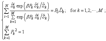 | (24) |
The above formula gives  equations with
  for
for  as the
  variables. Then the price victor
  can be solved by solving the above equation through many mature methods, such as Newton’s method [5, 9], Brent’s method [2, 13]. Thus all the micro supplies
  can be given through Equation (16), and all the macro supplies can be given through Equation (23) or Equation (17).
7.2. Solving the General Equilibrium as an Linear Programming Problem
The General Equilibrium Equation (23) can also be formulated as the following optimization problem: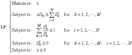 | (25) |
This is a linear programming problem with  and
and  as variables. It can be easily solved through the T-forward method [7, 8, 3]. Equation (24) and (25) should give the same solution.
8. Some Special Production Possibility Curves
In this section, we introduce two special scenarios with special production possibility curves. These curves can be used to compare with the PPF and can show how efficiency of the production states on the PPF.
8.1. Linear Production Possibility Frontier
We have introduced the micro vertex points as shown in Equation (5). A plane curve can be formulated by passing through these vertex points as following: | (26) |
Let us call this plane curve as the micro Linear Production Possibility Frontier (LPPF), and denoted as  . Similarly, we can construct a macro LPPF curve
  for the macro system
  , which can be formulated as:
 | (27) |
Using the price vector as a reference vector, the above equation can be expressed as: | (28) |
Note that the above Equation cannot be treated as the supply function, although it is expressed as functions of the price vector. It can be shown that: | (29) |
8.2. Self Sufficient Scenario
Another special scenario is the so called Self Sufficient case, in which every micro system just simply works on itself to provide all products with the amounts to be proportional to the requested demands. Within this scenario, there is no cooperation among micro systems. Let us call the PPF Curve for this scenario as SPPF. Let  and
and  be the micro SPPF and macro SPPF for the Self Sufficient scenario.
  is the same as the plane curve
  as shown in Equation (26). However, the macro SPPF
  is different from the Macro LPPF
  . By definition, given the requested demand as
  , the micro SPPF
  can be expressed as:
 | (30) |
And the macro SPPF  can be formulated as:
  | (31) |
9. A Dummy System with Dummy Data
In order to give concrete examples to demonstrate our model and methodology, let us create a dummy system with dummy data. The dummy system  is called the carpenter system, which contains
  units or members, and need to make
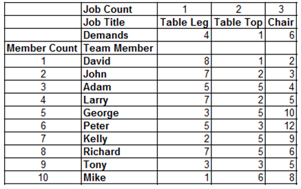
  products. The carpenter system needs to produce 4 table legs, 1 table top, and 6 chairs, which make up the 3 components of the demand vector. The micro capability matrix and demand vector are listed in Table 1. The requested amounts or demands are listed in row 3, and the production capabilities are listed in row 5 to 14.
Table 1. Input data for the carpenter system with 10 members and 3 products
 |
| |
|
Given the input data as listed in Table 1, by applying Equation (16), (26), and (30), the micro curves  ,
,  ,
,  , and
, and  are derived and are drawn in Figure 2. These four curves are all converged to the same plane curve.
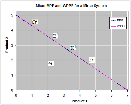 | Figure 2. The micro PPF , the micro WPPF , the micro WPPF  , the micro LPPF , the micro LPPF  , and the Micro SPPF , and the Micro SPPF  are all shown as the same plane curve in the production space are all shown as the same plane curve in the production space |
According to Equation (16), curves  and
and  could be different from the plane curve for some small
  . However, the difference can be only shown up for 3 or more dimensional case. If we set all other prices to 0 except two of them, then the above four curves always converge to the plane curve.Figure 3. shows the macro PPF
  , along with some other macro curves, including WPPF
  , LPPF
  , and SPPF
  . Figure 4 draws the supply-price curves for various
  value. By comparing with Figure 1, our model gives the PPF and supply functions in more detailed formats and make the general supply-demand equilibrium solvable numerically.
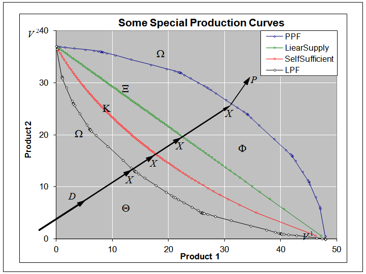 | Figure 3. The macro PPF  is a convex curve, the macro WPPF is a convex curve, the macro WPPF  and the macro SPPF and the macro SPPF  are concave curves, whereas the macro LPPF are concave curves, whereas the macro LPPF  is a linear plane curve in the production space. The maximum PPR is a linear plane curve in the production space. The maximum PPR  is the region bounded by is the region bounded by  and and  . The extension line of the demand vector . The extension line of the demand vector  intersects with these 4 curves at the points intersects with these 4 curves at the points  , ,  , ,  , and , and  respectively. These curves and points are used for improved efficiency analysis respectively. These curves and points are used for improved efficiency analysis |
10. The Best and the Worst Scenarios
Suppose each of the micro system  has reached its micro PPF
 , then the aggregated macro state of the macro system must be in the macro MPPR
 . Also, suppose the macro system
  is requested to produce the demand vector
 . The demand vector
  is as shown as the line
  in Figure 3. Figure 3. also shows the four points
 ,
,  ,
,  , and
, and , which are the intersection points of the line
  with the curves
 ,
,  ,
,  , and
, and . For all possible production states in
 , the Line
  gives all possible states that are proportional to the requested demand
 . Any other states in
  may have some products wasted or not needed compared with the requested demand
 . So, for all possible states in
 , only the states on line
  can best meet the requested demand
 . We are only interested in the states that are on the line
 . For all states on the line
 , the point
  is the best scenario, because it gives the maximum possible amount for all supplies,
  is the worst scenario, whereas
  and
and  are somewhere in the middle. Point
  can be treated as the average state for all points in the macro MPPR
 . Let us assume that point
  is the average state that the macro system reached without using any optimal management method. Now, let
  denote the improved production efficiency by comparing the best scenario
  with the average scenario
 , then
  can be formulated as:
 | (32) |
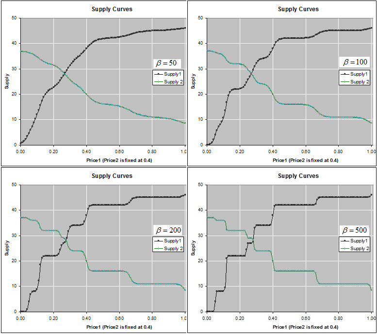 | Figure 4. Supply Curves. When price  rises and all other prices remain unchanged, the supply rises and all other prices remain unchanged, the supply  rises, whereas the supply for other products decreases, for example, Supply rises, whereas the supply for other products decreases, for example, Supply  decreases. When decreases. When  is large, the supply curves is large, the supply curves  and and  become step curves become step curves |
11. Application 1: Labor Assignment for Labor Oriented Team
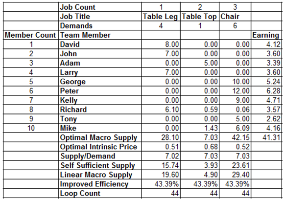
The mathematic formula for the Macro PPF and the supply function may have lot of applications and can improve the production efficiency significantly. Here we just introduce one of the applications of the macro PPF and the supply function: finding the optimal solution for team work management problems.We have developed a software tool that can find optimal solution for labor assignment problems by solving equation problem listed in Equation (24), or by solving linear programming problem as listed in Equation (25).By applying this software tool to the Carpenter team with the input data as listed in Table 1, we find the optimal solution as shown in Table 2. The solution given in Table 2 tells us at least the following information:Table 2. The optimal solution for the Carpenter team management problem
 |
| |
|
It tells all the information about the production state, including the amount of a production to be made by each team member. Each micro production state is a point on the corresponding micro PPF.Most of the team members should work on only one product. Some of the team members may work on multiple products. For example, team member David should work only on “Table Legs” and make 8 “Table Legs” within requested time T, while Richard should work on all 3 products, and make 6.1 “Table legs”, 0.59 “Table Tops”, and 0.06 “Chairs”. The final macro Supply is 28 “Table legs”, 7 “Table Tops”, and 42 “Chairs”. This macro Supply state is on the macro PPF  and proportional to the requested production demand vector
  . The last column gives the Earnings or Incomes for each team member.The row with header “Supply/Demand” gives the number
 defined in Equation (23). It is the ratio between the optimal solution and the requested demand amount.The row with header “Optimal Intrinsic Price” gives the intrinsic prices which can be used to calculate the earnings for each team member. The intrinsic price vector for these 3 products should be (0.51, 0.68, 0.52). Once this intrinsic price vector is known, each team member will reach his maximum income by making the products with the amounts as requested in the optimal solution. In other words, the whole team will realize the optimal solution automatically as long as each sub unit has maximized its income.The row with header “Self Sufficient Supply” lists the supply state
  on the SPPF
  . The row with header “Linear Macro Supply” lists the supply state
  on the LPPF
  . The row with header “Improved Efficiency” lists the improved efficiency ratio by the optimal solution
  compared with the Linear Macro Scenario
 . The row with header “Loop Count” lists the number of loops for our numerical calculation to converge to the results with required precision. The optimal solution not only depends on the capability matrix, but also depends on the direction of the demand vector. Given a team member and his capability matrix, we cannot tell which product is the most specialized product for him. The optimal solution may request him to work on one product. However, once the direction of the demand vector changes, the same team member might be requested to work on some other products to have the whole team to reach the optimal solution.
12. Application 2: Labor Assignment for Project Oriented Team
Application 1 gives an example of a team working on products, which is more applicable to a labor oriented team. A product oriented team is basically a team working on products and the demands can be simply formulated as the amounts of the products. A project oriented team is a team working on projects, while each project is required to be delivered in a given deadline. For a project oriented team, the capability parameter  can be explained as the delivery ratio (or amount) of the kth project
  by team member
  . The demand for each project is 1 within required delivery time. Let
  denote the required delivery time for the kth project
  , and
, and  denote the fastest delivery time of team member
  to deliver the kth project
  under the condition that
  works only on project
  . Then the equivalent demand vector can be expressed as:
 | (33) |
And the equivalent production capability parameters can be expressed as: | (34) |
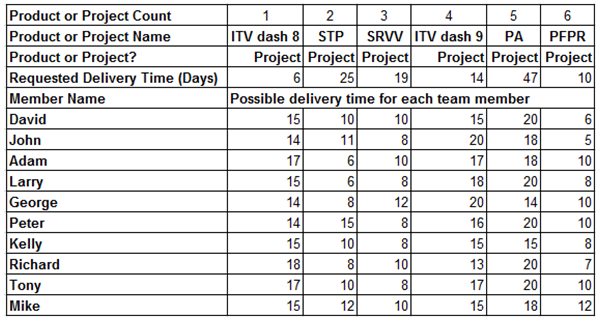
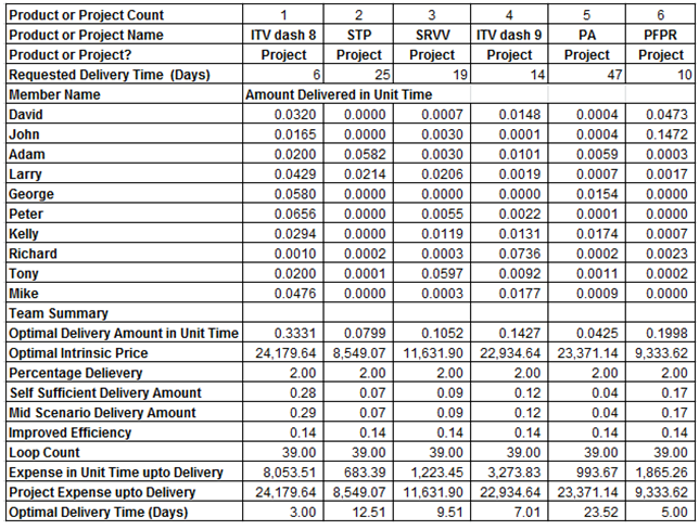
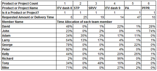
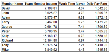
Then, our proposed model for labor assignment is applicable to project oriented teams. We have applied our proposed model to manage an engineer team in Boeing Corporation. Let us call this team as Boeing team. The Boeing team includes 10 Engineers to work on 6 projects that need to be delivered in requested deadlines. The total budget for these projects is 100,000 USD. Table 3 lists the fastest delivery time for each team member to deliver each project. If we inverse each number in this table, it will be the capability parameter matrix. Please note that we have given dummy names for each team member. The Boeing Team was given a strict deadline to finish these projects. The manager had been worried about whether they could deliver these projects and struggled for labor assignment among the team members. By solving Equilibrium Equation (24), or solving the linear programming problem as listed in Equation (25), we can give the optimal labor assignment solution for the Boeing team. Table 4 lists the amount to be delivered in unit time for each team member and each project. Table 5 lists the optimal assignment in terms of time allocation for each team member. Table 6 lists the income, total work days, and the pay-rate for each team member. With our optimal solution for labor assignment, the Boeing Team can deliver all of their 6 projects on time and all the actual delivery time are reduced by half compared with the original requested delivery time. Table 3. The delivery capability matrix and requested delivery time for Boeing team
 |
| |
|
Table 4. The optimal solution for a project oriented team in Boeing Corporation
 |
| |
|
Table 5. Optimal Time allocation for a project oriented team in Boeing Corporation
 |
| |
|
Table 6. Income and pay rate at the Equilibrium state
 |
| |
|
13. Production Efficiency Improvement for the Carpenter Team
Note that, even with the worst scenario case, all team members have worked hard to reach their micro PPF states. In other words, although all team members have exhausted all of their resources to work on the requested products, the production output are very different for the macro system. The inefficiency for the worst scenario is completely due to improper management. With proper arrangement, we can have the team to improve production efficiency by 148% compared with the worst scenario.Table 7 lists the macro supplies for the optimal solution, the worst scenario solution, the Linear Macro Supply scenario, as well as the Self-Sufficient scenario. It also lists the improved production efficiency ratios by comparing with the Self-Sufficient scenario as well as the Linear Macro Supply scenario. Table 7. Improved Production Efficiency Ratios for the Carpenter Team
 |
| |
|
By comparing with the Self-Sufficient Supply scenario, we can find out how much efficiency improved due to the division of labors and corporations among team members. The Linear Macro Supply scenario can improve the production efficiency by 25%, whereas our optimal solution can improve the production efficiency by 79%. These improved efficiencies come from the division of labor and cooperation among team members. Some managements with good quality are required to realize such kind efficiency improvements. Our proposed method gives the optimal solution for team work management. By comparing with the supply state  , we can find the improved efficiency ratio by the optimal solution. The improved efficiency for the carpenter team is:
 | (35) |
14. Estimate the Improved Production Efficiency for Generic Cases
As discussed in the previous sections, by applying our optimal management method, the Carpenter team can improve its production efficiency by 43%. That is amazing! However, people might argue that the Carpenter team is just a special case. In this section, we estimate the production efficiency improvement ratio that can be brought by the optimal solution for generic cases. Our analysis shows that the optimal solution can really improve production efficiency by 40% for most of the team work management problems.To simplify our analysis, we assume the demand vector as  in this section. Let
  be the intersection point of the demand vector
  (or its extension) with the curve
  , and
, and  denote the length of the line
  . Then
  can be easily found as:
 | (36) |
As the macro PPF  is a convex curve, we can use
  to approximate the PPF
  , with
  to be a value that can make the
  most close to
  . Normally, once we find one point on
  , we can calculate the value of
  which can make the
  most close to the
  . Further, we assume the average production state is roughly at the point
  on the curve
  (or denoted as
 ). If
). If  is used to approximate
  , the improved efficiency by reaching the macro PPF can be estimated as:
 | (37) |
Actually, the more team members the team has, the more convex the macro PPF tends to be. Based on our test results, we found that  is a good approximation for
  when
when ; and even
  will be a good approximation for
  when
when  and
and . To make it more conservative, we use
  to approximate the macro PPF
 . Then the production efficiency ratio that can be improved by the optimal solution can be estimated as:
 | (38) |
Table 8 lists the possible production efficiency improved by the optimal solution for a team working on  products. Based on our test results and the above analysis, our optimal solution for team work management normally can improve the production efficiency by 40% for most of team work problems!
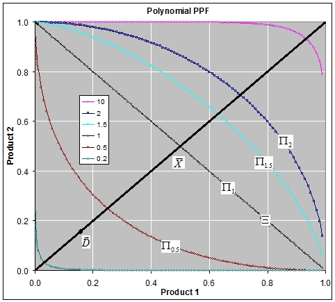 | Figure 5.  can be used to approximate the PPF can be used to approximate the PPF  and LPPF and LPPF  . Here all the curves are shown in 2-dimensional. You need to imagine it in M-dimensional . Here all the curves are shown in 2-dimensional. You need to imagine it in M-dimensional |
Table 8. Production Efficiency Improved by the Optimal Solution for a Team
 |
| |
|
15. Micro and Macro Management
By applying the proposed method and the software tool, we can find the optimal solution for the team work management, or labor assignment problems. Suppose you are the team manager, how are you going to manage your team to reach the optimal management? Here we propose two management methods: Micro Management and Macro Management.
15.1. Micro Management
Our optimal solution for team work management problems, as shown in Table 2 and Table 4, lists all the micro information for each team member, including micro supply amount  , and the micro income amount
  . Using these micro information, a team manager can tell each team member
  to work on the
  with the amount
  as indicated in the optimal solution. Note that most of the team members may work on only one product. The team manager can also tell each team member
  about how much he should be paid, which would be
  . So, with micro management, a team manager manages each of the team members in micro details, including what and how much need to be done, as well as how much should be paid as return. That is why we call this management method as Micro Management.
15.2. Macro Management
Our optimal solution for team work management problems, as shown in Table 2 and Table 4, also gives the intrinsic prices  . Given this intrinsic price vector, each team member will reach his maximum income by working on the product with the amount as requested by the optimal solution. Suppose each team member is targeting at maximizing his income, the team manager needs only declare the intrinsic prices, then, every team member will automatically to work on the product with the amount such that the whole team will reach its optimal solution as indicated in the optimal solution. The team manager doesn’t manage the team members in micro details, but manage it in macro level, which simply tells how much will be paid for product or project to be delivered. That is why we call this management method as macro management.
16. Conclusions
The main contributions of this paper include a new model that can formulate the Supply function and the Production Possibility Frontier as a function of the capability parameters and the price vector. The Law of Supply, the supply elasticity can be easily derived from the proposed model. Another contribution is the methods for solving the Supply-Demand equilibrium. Lastly, we present a model and method that can give optimal solution for labor assignment and team work management problems based on the Supply-Demand equilibrium. Our test results and generic analysis show that the proposed management method can improve the team work efficiency significantly. For most cases, it can improve the production efficiency by 40%!
References
| [1] | [Bar10] R. R. Barthwal, Industrial Economics: An Introductory Textbook. P. 31, 2010. |
| [2] | [Bre73] R. P. Brent. Algorithms for Minimization without Derivatives. Chapter 4. Englewood Cliffs, NJ: Prentice-Hall, 1973. ISBN 0-13-022335-2. |
| [3] | [DS97] Robert Dorfman; Paul A. Samuelson; Robert M. Solow. Linear Programming and Economic Analysis. McGraw-Hill College Division, 1997. ISBN: 0486654915. |
| [4] | [Gil07] Andrew Gillespie, Foundations of Economics. Ch. 2. Oxford University Press, 2007. |
| [5] | [Kel03] C. T. Kelley, Solving Nonlinear Equations with Newton's Method, no 1 in Fundamentals of Algorithms, SIAM, 2003. ISBN 0-89871-546-6. |
| [6] | [Liu02] G. Liu, Analytic Economics, P. 39-90, 2002. ISBN 10: 0971893403 / ISBN 13: 9780971893405. |
| [7] | [Liu14] G. Liu, “T-Forward Method: A Closed-Form Solution and Polynomial Time Approach for Convex Nonlinear Programming”. Algorithms Research, Vol.3, No.1: 1-23. 2014. |
| [8] | [Liu14] G. Liu, “T-Forward Method: A Closed-Form Solution and Polynomial Time Approach for Convex Quadratic Programming”. Applied Mathematics, 2014. |
| [9] | [OR00] J. M. Ortega, W. C. Rheinboldt, Iterative Solution of Nonlinear Equations in Several Variables. Classics in Applied Mathematics, SIAM, 2000. ISBN 0-89871-461-3. |
| [10] | [PR09] Robert Pindyck, Daniel Rubinfeld, Microeconomics, The Pearson Series in Economics, 2012. ISBN-10: 013285712X / ISBN-13: 978-0132857123. |
| [11] | [Sam04] Paul A. Samuelson and William D. Nordhaus, Economics. Chapter 1-5.McGraw-Hill; 16th Edition, 1998. ISBN 7-111-06448-8. |
| [12] | [Sam67] Paul A. Samuelson. “Summary on Factor-Price Equalization”. International Economics Review, Vol. 8, No. 3, 8(3): 286-295, 1967. |
| [13] | [Sta13] Steven A. Stage. “Comments on An Improvement to the Brent's Method”, International Journal of Experimental Algorithms 4 (1): 1–16.2013. |

 : An economic system that contains some sub systems. It can be as small as a family, a firm, and can be as large as a country or the whole world.
  is also called a macro system compared with its sub systems.
 : An integer represents the total number of the sub systems in
  .
.  : An integer represents the total number of the products that are produced in
  .
.  : The ith unit or sub system in system
  . It could be an individual member, or a group of people, such as a firm or another economic system in
  . However, there are no overlaps between different Units. For example, if an individual has been included in one unit, the same individual can’t be included in another unit.
  is also called a micro system compared with its parent system.
 : The kth product that can be produced in system
  . Actually, the product here means any labor activities that can be done by any unit in
  . It can be a real product, a project, a job, a task, and anything that need to be done or produced by any unit in
  .
. : A time span that the above mentioned products are produced in
  .
. :
:  , which is the set of non-negative M-dimensional real vectors and with the original point
  excluded.
 : The same as
  . However, we use it to particularly represent the Production Space with its kth Cartesian coordinate representing the amount of a parameter related to
  product.
 : The demand amount of
  product that requested by
  .
.  : The maximum amount of
  product that can be produced by
  within time
  . Normally
  can be produced by
  when it uses all of its resources to work on product
  . All the
  make up an
  matrix, which is called the micro capability matrix of system
  .
.  : The amount of
  product that are actually produced by
  . All the
  make up a vector in
  , and is called micro supply vector.
 : The amount of
  product produced by the macro system
  . It is also called the macro supply of system
  . All the
  make up a vector in
  , and is called a macro supply vector of system
  .
. ;
;  : The price of the
  product in system
  .
. introduced above. An economic system is called a micro system if it is contained in a macro system, such as the sub-system
  described above. Definition: System Parameter: An economic parameter is called a system parameter if it is associated with an economic system. For example, the supply amount, demand amount, and price are all examples of system parameters. Definition: Micro Parameter and Macro Parameter: A system parameter is called a micro parameter if it is associated with a micro system, and is called a macro parameter if it is associated with a macro system. Some parameters may be associated with both micro system and macro system. As long as there is no confusion, we use the same alphabet character to represent a system parameter: if
  denotes a macro parameter associated with a macro system
  , then
  will be used to denote the same micro parameter associated with micro system
  .For example,
  and
and  represent the macro and micro supply amounts of product
  ,
,  and
and  denote the macro PPF of system
  and the micro PPF of the micro system
  correspondingly. Definition: Vector Parameter and Scalar Parameter: a system parameter may also be associated with each of the production, for example, supply amount normally means the amount of a product that can be provided by an economic system. In a system with
  products, a system parameter could be
  -dimensional with each component representing the amount associated with one product. These
  -dimensional parameters make up a vector in the production space
  , thus is called a Vector Parameter. A vector parameter can be represented by a vector in
  . Examples of vector parameters are: Supply, Demand, and Price. A system parameter is called a scalar parameter if it is one dimensional. Examples of scalar parameters are: income, GDP, revenue, etc.Additive Parameter: A system parameter is called additive parameter if the corresponding macro parameter can be derived by aggregating the same parameter over all of its micro systems. Or precisely, system parameter X is additive if
 is a parameter reachable and meaningful to micro system
  , while
  is the same parameter reachable and meaningful to macro system
  .In our model, we tried to decompose the macro system
  into some micro systems
  , and divide the products into some products or tasks in such a way that some of the system parameters are additive, particularly, the supply amount, the demand amount, revenue, and income are all additive. However, the price parameter is not an additive parameter. Based on the above notations and definitions, we can say that the supply and demand are vector parameters and are additive, whereas the price is also a vector parameter, but not additive. The income, revenue, GDP, profit and loss are all additive scalar parameters. We are only interested in those parameters in this paper.
  , the production capability matrix for each micro system and for each product.
 : The macro demand of
  product that needs to be accomplished by system
  . We assume the following parameters are unknowns and need to be resolved: Price, micro supply, macro supply, micro income, macro revenue.
  , let us assume that it can arrange its resources to make any requested products. However, its production amount for product
  should be limited to or bounded by
  due to its limited resources and capabilities. Any of its feasible production state will be a point or a vector in the production space
  . All of its feasible production vectors should be a bounded range in the production space
  . We call this bounded range as its micro Production Possibility Range (PPR) and denoted as
  . The upper boundary of
  is called the micro PPF, denoted as
  . Normally, as long as the micro system
  is small enough compared with macro system
  , each of the micro PPF can be approximated by the linear plane curve that passing the
  axis at
  in production space
  . Given the micro capability matrix, the micro PPF
  can be formulated as:
 can also be expressed in the following format:

 is called the intrinsic price vector of the micro system.Actually,
  is a linear plane curve with vector
  as its normal vector. It passes the
  axis at the points:
 is the unit vector on the
  axis.
axis.  and is on the
  axis of the production space. We call these
  points as the micro vertex points. Given the price vector as
  and the micro supply vector
  of the micro system
  , the total income or revenue of the micro system
  can be expressed as:
 is feasible to micro system
  , there should have some possible micro supply vectors that can maximize the income or revenue of the micro system
  . Such feasible micro supply vectors can be formulated as:
 to be maximized is a linear function, according to Lagrange’s theorem, the max-min can only be found on the boundary of the region
  . Then the above equation is equivalent to:
 vertex points listed in Equation (5). Then, the above equation can be further simplified as:

 is an
is an  function defined as:
 is the total number of vertex points that have
  maximized for
  . Number
  can be formulated as:

 maximized. It gives at least one of the micro supply vectors
  that can have the micro income
  maximized. It is an explicit mathematical format for the micro supply as a function of the capability matrix and the price vector. However, it is a discrete function and thus is difficult to deal with. The key step and major contribution of our model is to formulate a continuous and smooth function to approximate the Equation (13). Here are the key steps. Equation (13) is equivalent to the following function:
 is called the macro capability parameter defined as:
 . In practical applications, we can simply drop the limited function by assigning
  with a large number, thus the Equation (14) can be simply expressed as:
 for
for  ; Normally, it will be good enough if we assign
  as:
as: Equation (16) will be a good approximation for the micro supply function, and it gives the Micro PPF
  once the price vector goes through all possible directions in the production space
  .
.  will be good enough for most of the practical applications. We use
  to get most of the results listed in this paper.
  and the micro supply as a function of the price vector and the capability parameters, as shown in Equation (16). As each of the micro system
  has a maximum production frontier and a limited range as its PPR, the macro system should also have a macro PPR in the production space
  , and must have a macro PPF. As the supply parameter is an additive parameter, we can get the macro supply vector by aggregating all the micro supply vectors, that is:
 , as shown in Figure 3. So, the above Equation is not only a supply function, but also a function that gives the macro PPF
  . Figure 4.shows the Supply-Price curves for various
  values. Once
  is big enough, the Supply-Price curves become step curves. Keeping in mind that each micro system is targeting at maximizing its income, so, when the price
  rises, a micro system
  may want to switch all of its resources to work on product
  , and thus to have the macro supply
  be suddenly increased by an amount of
  . At the same time, because
  switched from working on
  to work on some other products, such as
  (
( ), it will have the supply
  decreased suddenly by an amount of
  . This explains why the Supply-Price curve shows as a step curve, also explained the Law of Supply as discussed in later sections. The supply functions and the PPF given in Equation (17) are the key contributions of this paper. The rest of the paper discusses applications of this supply function, or compare our PPF with some other production possibility frontiers and see how much efficiency can be improved by using our proposed model.
 denote the micro WPPF of micro system
  , and
, and  denote the macro WPPF of the macro system
  .
.  is defined as the lower boundary under the conditions that all of its micro systems have reached their micro PPF
  . The WPPF
  is defined as the set of micro supply vectors that are on the
  and results a macro supply vector on the macro WPPF
  if aggregated for all micro systems.
  and
and  can be formulated using the same Equations as shown in Equation (16) and (17), as long as we set
  . We will not rewrite these Equations here. Let
  be the region bounded by
  and
and  , and
, and  be the region bounded by
  and
and  .
.  is called the micro Maximum Production Possibility Range (MPPR), and
  is called the macro MPPR. Given a price vector
  , through Equations (16) and (17),we can get a macro supply vector
  on
on  , a macro supply vector
  on
on  , a micro supply vector
  on
on  , and a micro supply vector
  on
on  . It can be shown that the price vector
  is the normal vector of those curves at the corresponding points as indicated by these supply vectors [6].
 denote the supply elasticity for the
  product. By applying partial differentiation to Equation (16) and (17), we can easily have:


 given in Equation (19) is non-negative. Noting that
  and
and  , thus all items in Equation (19) is non-negative, then the elasticity
  which is a sum of some non-negative numbers is also non-negative. Thus Equation (20) is proven. By applying partial differentiation to Equation (16), we have:
 ,
,  , for
, for  and
and  Equation (21) follows the above two equations immediately, and thus the Law of Supply is proven.
 and
and  are functions of
  . Thus, the above general equilibrium equation gives
  equations with
  prices as unknowns. Generally, once we know the function format for
  and
and  , the equilibrium price vector can be solved from Equation(22). We do not try to give a generic format for demand functions in this paper, instead, we just simply assume the demand is given as a vector with fixed direction, thus Equation (22) can be expressed as:

 equations with
  for
for  as the
  variables. Then the price victor
  can be solved by solving the above equation through many mature methods, such as Newton’s method [5, 9], Brent’s method [2, 13]. Thus all the micro supplies
  can be given through Equation (16), and all the macro supplies can be given through Equation (23) or Equation (17).
 and
and  as variables. It can be easily solved through the T-forward method [7, 8, 3]. Equation (24) and (25) should give the same solution.
 . Similarly, we can construct a macro LPPF curve
  for the macro system
  , which can be formulated as:


 and
and  be the micro SPPF and macro SPPF for the Self Sufficient scenario.
  is the same as the plane curve
  as shown in Equation (26). However, the macro SPPF
  is different from the Macro LPPF
  . By definition, given the requested demand as
  , the micro SPPF
  can be expressed as:
 can be formulated as:
 is called the carpenter system, which contains
  units or members, and need to make
  products. The carpenter system needs to produce 4 table legs, 1 table top, and 6 chairs, which make up the 3 components of the demand vector. The micro capability matrix and demand vector are listed in Table 1. The requested amounts or demands are listed in row 3, and the production capabilities are listed in row 5 to 14.
 ,
,  ,
,  , and
, and  are derived and are drawn in Figure 2. These four curves are all converged to the same plane curve.
 , the micro WPPF
  , the micro LPPF
  , and the Micro SPPF
  are all shown as the same plane curve in the production space
 and
and  could be different from the plane curve for some small
  . However, the difference can be only shown up for 3 or more dimensional case. If we set all other prices to 0 except two of them, then the above four curves always converge to the plane curve.Figure 3. shows the macro PPF
  , along with some other macro curves, including WPPF
  , LPPF
  , and SPPF
  . Figure 4 draws the supply-price curves for various
  value. By comparing with Figure 1, our model gives the PPF and supply functions in more detailed formats and make the general supply-demand equilibrium solvable numerically.
 has reached its micro PPF
 , then the aggregated macro state of the macro system must be in the macro MPPR
 . Also, suppose the macro system
  is requested to produce the demand vector
 . The demand vector
  is as shown as the line
  in Figure 3. Figure 3. also shows the four points
 ,
,  ,
,  , and
, and , which are the intersection points of the line
  with the curves
 ,
,  ,
,  , and
, and . For all possible production states in
 , the Line
  gives all possible states that are proportional to the requested demand
 . Any other states in
  may have some products wasted or not needed compared with the requested demand
 . So, for all possible states in
 , only the states on line
  can best meet the requested demand
 . We are only interested in the states that are on the line
 . For all states on the line
 , the point
  is the best scenario, because it gives the maximum possible amount for all supplies,
  is the worst scenario, whereas
  and
and  are somewhere in the middle. Point
  can be treated as the average state for all points in the macro MPPR
 . Let us assume that point
  is the average state that the macro system reached without using any optimal management method. Now, let
  denote the improved production efficiency by comparing the best scenario
  with the average scenario
 , then
  can be formulated as:
 and proportional to the requested production demand vector
  . The last column gives the Earnings or Incomes for each team member.The row with header “Supply/Demand” gives the number
 defined in Equation (23). It is the ratio between the optimal solution and the requested demand amount.The row with header “Optimal Intrinsic Price” gives the intrinsic prices which can be used to calculate the earnings for each team member. The intrinsic price vector for these 3 products should be (0.51, 0.68, 0.52). Once this intrinsic price vector is known, each team member will reach his maximum income by making the products with the amounts as requested in the optimal solution. In other words, the whole team will realize the optimal solution automatically as long as each sub unit has maximized its income.The row with header “Self Sufficient Supply” lists the supply state
  on the SPPF
  . The row with header “Linear Macro Supply” lists the supply state
  on the LPPF
  . The row with header “Improved Efficiency” lists the improved efficiency ratio by the optimal solution
  compared with the Linear Macro Scenario
 . The row with header “Loop Count” lists the number of loops for our numerical calculation to converge to the results with required precision. The optimal solution not only depends on the capability matrix, but also depends on the direction of the demand vector. Given a team member and his capability matrix, we cannot tell which product is the most specialized product for him. The optimal solution may request him to work on one product. However, once the direction of the demand vector changes, the same team member might be requested to work on some other products to have the whole team to reach the optimal solution.
 can be explained as the delivery ratio (or amount) of the kth project
  by team member
  . The demand for each project is 1 within required delivery time. Let
  denote the required delivery time for the kth project
  , and
, and  denote the fastest delivery time of team member
  to deliver the kth project
  under the condition that
  works only on project
  . Then the equivalent demand vector can be expressed as:

 , we can find the improved efficiency ratio by the optimal solution. The improved efficiency for the carpenter team is:
 in this section. Let
  be the intersection point of the demand vector
  (or its extension) with the curve
  , and
, and  denote the length of the line
  . Then
  can be easily found as:
 is a convex curve, we can use
  to approximate the PPF
  , with
  to be a value that can make the
  most close to
  . Normally, once we find one point on
  , we can calculate the value of
  which can make the
  most close to the
  . Further, we assume the average production state is roughly at the point
  on the curve
  (or denoted as
 ). If
). If  is used to approximate
  , the improved efficiency by reaching the macro PPF can be estimated as:
 is a good approximation for
  when
when ; and even
  will be a good approximation for
  when
when  and
and . To make it more conservative, we use
  to approximate the macro PPF
 . Then the production efficiency ratio that can be improved by the optimal solution can be estimated as:
 products. Based on our test results and the above analysis, our optimal solution for team work management normally can improve the production efficiency by 40% for most of team work problems!
 can be used to approximate the PPF
  and LPPF
  . Here all the curves are shown in 2-dimensional. You need to imagine it in M-dimensional
 , and the micro income amount
  . Using these micro information, a team manager can tell each team member
  to work on the
  with the amount
  as indicated in the optimal solution. Note that most of the team members may work on only one product. The team manager can also tell each team member
  about how much he should be paid, which would be
  . So, with micro management, a team manager manages each of the team members in micro details, including what and how much need to be done, as well as how much should be paid as return. That is why we call this management method as Micro Management.
 . Given this intrinsic price vector, each team member will reach his maximum income by working on the product with the amount as requested by the optimal solution. Suppose each team member is targeting at maximizing his income, the team manager needs only declare the intrinsic prices, then, every team member will automatically to work on the product with the amount such that the whole team will reach its optimal solution as indicated in the optimal solution. The team manager doesn’t manage the team members in micro details, but manage it in macro level, which simply tells how much will be paid for product or project to be delivered. That is why we call this management method as macro management.
 Abstract
 Reference
 Full-Text PDF
 Full-text HTML


 is a convex curve, the macro WPPF
  and the macro SPPF
  are concave curves, whereas the macro LPPF
  is a linear plane curve in the production space. The maximum PPR
  is the region bounded by
  and
and  . The extension line of the demand vector
  intersects with these 4 curves at the points
  ,
,  ,
,  , and
, and  respectively. These curves and points are used for improved efficiency analysis
 rises and all other prices remain unchanged, the supply
  rises, whereas the supply for other products decreases, for example, Supply
  decreases. When
  is large, the supply curves
  and
and  become step curves