1. Introduction

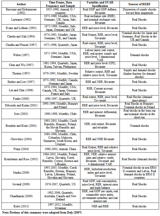
By definition, the exchange rate is the domestic currency price of a foreign currency. Within the context of Ghana, the real effective exchange rate is also a measure of the rate of exchange of the cedi relative to a trade-weighted average of Ghana’s trading partners' currencies. Foreign exchange rates are one of the most important determinants of a country’s relative level of economic health, playing a fundamental role in trade, investment and financial transactions. Since Ghana moved to a market determined foreign exchange regime in the mid-1980s as part of the economic recovery and structural adjustment programme, the effects of dramatic movement of exchange rates have continued to generate series of responses. Ghana has witnessed some impressive economic performance over the past ten to fifteen years, even though a number of structural challenges still limit the economy. Ghana is today one of the best-performing economies in Africa. Starting from a very low base in 1980s, Ghana has quickly moved to high GDP growth and falling inflation, in conjunction with serious efforts towards market reforms. In between the years, the policy arena became primarily characterized by high and volatile inflation and exchange rate depreciation. For some other years, Ghana witnessed strong fiscal dominance in which persistent fiscal deficits were financed largely by monetary accommodation [1].

Attention in recent years has been directed at strengthening the role of monetary policy aimed explicitly to achieve price stability and operationalized through the adoption of an inflation targeting regime[1]. The new BOG Act, 2002, (Act 612) set the tone for inflation targeting (IT) in Ghana. Section 27 of the Act provides for the establishment of a Monetary Policy Committee chaired by the governor of the Bank of Ghana who has a vote and supported by six other independent members in the decision process. Also, the Act tackles the issue of fiscal dominance by placing a limit on government’s borrowing in any fiscal year. The monetary policy framework under this new Act has been designed to engineer a switch to low inflation and exchange rate stability, through increased coordination with fiscal policy[1].

Given that policy coordination is critical in the inflation targeting process, it would be worthwhile to examine systematically, using time-series econometric techniques, the interactions between the key indirect instruments of monetary control. This study focuses on the real effective exchange rate and examines the underlying forces that drive real exchange fluctuations over the past two decades. Specifically, the study adopts an unrestricted vector autoregression (VAR) model to estimate the relative importance of three types of shocks namely: aggregate supply shocks, aggregate demand shocks and nominal demand shocks. The approach allows for the decomposition of fluctuations in real effective exchange rate into various components and measures the relative importance of each of the components. The study is similar in spirit and conception to earlier works by[2] for Myanmar,[3] for Croatia,[4] for the US,[5] for Canada,[6] for Tunisia,[7] for Turkey,[8] for China,[9] for South Africa, and[10] for Poland and Hungary. Other related studies include those by[11],[12],[13] and[14].¹

Unfortunately, the results of these referred studies do not point to an unambiguous answer to the question whether the real exchange rate acts as a shock absorber or as a source of shocks. All the studies differ regarding the type of data used, the period of analysis, the number of variables used (which also dictates the number of shocks that can be identified) and model specification. This leads to the conclusion that the results of the studies are specification sensitive and one has to be very cautious with their interpretation. Again, though the existing literature is extensive, similar empirical analysis based on Ghana are scanty, hence the motivation to test the unrestricted VAR model using new data and examine whether its predictions apply in the case of Ghana. As is generally known, monetary policy is a dynamic process that needs to be occasionally adjusted to reflect prevailing conditions. The findings allow us to gauge the effectiveness of real and nominal shocks in the country and judge the ability of policymakers to affect real exchange rates through adherence to nominal anchors.

The rest of the paper is organized as follows. In the next section, an overview of foreign exchange developments is provided. This is followed up in section 3 by a discussion of the theoretical framework that guides the relationship between foreign exchange rate, price levels and real output. The methods used together with the data sources are discussed in section 4. In Section 4, the empirical findings including the results from unit root tests, forecast error variance decomposition and impulse response functions are presented. The last section provides the conclusions and policy implications from the study.

2. Foreign Exchange Developments in Ghana

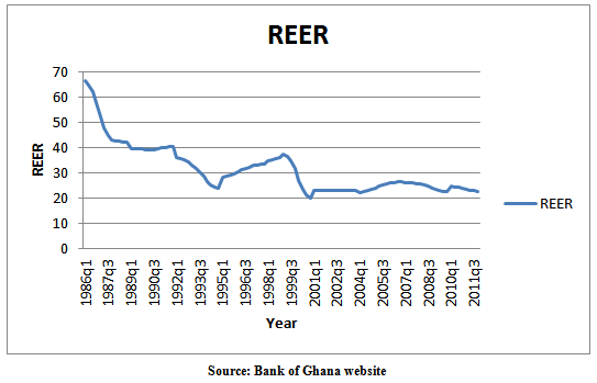
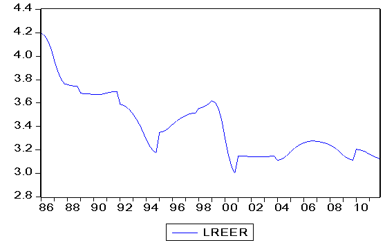
The exchange rate policy in Ghana has been one of the most significant policy reforms which began in the mid 1980s as part of the economic recovery and structural adjustment programme. Foreign Exchange Reforms in Ghana involved an initial devaluation of the local currency, the operation of a two-tier system in September 1986 and the eventual and complete liberalization of the foreign exchange market and rate regime in 1988. The operation of the two-tier system comprised of a higher officially determined rate and the auction rate. The officially determined rate applied to imports of petroleum and essential drugs, cocoa exports and debt service. The auction rate, on the other hand, applied to other transactions and was based on an auctioning conducted by the Bank of Ghana. Building on the measures taken during the economic recovery phase, the auction and official rates of exchange were unified in February 1987. Over the 1987-1988 period access to the auction was progressively widened to include all current transactions. By February 1988, there were effectively no restrictions on the import of goods except for five items on a “negative list” and expanded to include all bonafide requests for the transfer of profits and dividends. In December of the same year authorized dealer banks and eligible foreign exchange bureaus were given the responsibility of determining the eligibility of individual bids for foreign exchange. In April 1990, the auction was transformed from retail to a wholesome market and interbank foreign exchange transactions were authorised. Eligible banks and bureaus could bid and dealers could trade among themselves in interbank market and were free to retail at rates negotiated with buyers. The foreign exchange market adjusted smoothly to these structural reforms.

The exchange rate policy in Ghana has focused on achieving a stable exchange rate. Ghana’s exchange rate policy is based on reserve targeting. In instances where foreign exchange reserves were higher than targeted, the Bank of Ghana engaged in an outright sale of foreign currency to stabilise the exchange rate and to mop up excess liquidity in the system. The Bank of Ghana also engages in foreign exchange swap to influence domestic liquidity, manage foreign exchange reserves, and stimulate domestic financial markets. When the central bank buys forex in a swap with domestic currency, it injects liquidity into the market, similar to repo. The figure below indicates the movements in quarterly real effective exchange rates from January 1986 to December 2011. As evident, the cedi tends to depreciate against major currencies in the world for most of the period under consideration. Even though exchange rate fluctuations have significantly reduced in recent years in Ghana, the effects of a number of shocks remain noticeable even if muted[1].

3. Theoretical Foundations

The theoretical framework that guides this study is rooted in the[15] and[16] small open macro model which attempts to capture the dynamics of relative output, the real exchange rate and relative prices. The model is made up four equations which are reproduced below as outlined in the papers by Daly[6],[17] and[18].

(1)

(2)

(3)

(4)

Equation (1) is an open economy IS equation in which the demand for home output relative to foreign output () depends positively of the real exchange rate ( ) and the relative demand shock () and negatively of the real interest differential in favour of the home country. Equation (2) is a price setting equation in which the price level in period t is an average of the market clearing price expected in t-1 to prevail in t and the price that would clear the output market in period t. Equation (3) is a standard LM equation where relative real money balances are positively related to relative output and negatively related to the relative level of the interest rate. The relative interest rate ( ) in equation (4) is determined according to the interest parity condition where is the nominal exchange rate.

The key assumptions of the model include (i) prices and output adjustments are sticky and sluggish (ii) foreign and domestic goods are imperfect substitutes in consumption. The theoretical model above has important implications for short and long-run effects of the disturbances that have proved useful for empirical application. Shocks in the model can be categorized into aggregate supply shocks, such as changes in the relative productivity of home to foreign countries; aggregate demand or absorption shocks, such as changes in relative government spending and relative market access for home versus foreign products; and nominal shocks such as monetary policy shocks, money demand shocks (e.g., velocity shifts), and effects of financial liberalization. Consistent with standard macroeconomic models with sticky prices, in the short run real demand disturbances and nominal disturbances have only a short-run impact on output and are neutral in the long-run. Therefore, only supply shocks are expected to have an impact on the level of relative output in the long run. Also, supply and demand shocks are expected to influence the long run level of real exchange rate. Finally, both real supply shocks and nominal monetary shocks are expected to influence the long run level of prices. A commonly used econometric framework that has been used over the years to operationalize the[11] theoretical framework is the Vector Autoregression (VAR) model.¹

4. Methodology

4.1. The Unrestricted Multivariate VAR Framework

Following earlier works by[8],[6] and[3], this study employs a trivariate unrestricted VAR model and examines how each variable has contemporaneous effect on the other. The three variables are consumer price index (representing aggregate demand shock), real GDP (an aggregate supply shock) and the real effective exchange (a nominal shock). The typical VAR multivariate framework assumes that changes in a particular variable are related to changes in its own lags and to changes in other variables and the lags of those variables. The VAR treats all variables as jointly endogenous and does not impose a priori restrictions on the structural relationships. Because the VAR expresses the dependent variables in terms of only predetermined lagged variables, the VAR model is a reduced form model which can be expressed in the form below:

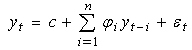(5)

where is a (nx1) vector of all the 3 variables in the system, c = (c1,…,c3) is the (3x1) intercept vector of VAR, is the (3x3) matrix of autoregressive coefficients for I=1,2,…p, and the (3x1) generalization of a white noise process. The vector autoregressive model is estimated in levels of the variables in natural logarithms. The VAR system in equation can be transformed into a moving average (MA) representation in order to analyze the system's response to shocks of selected variables. This is represented as is:

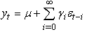(6)

Figure 1. Quarterly Trends in Real Effective Exchange Rate (1986-2011)

where is the identity matrix, is the mean of the process. The representation of the VAR system allows us to analyze the impact of one unit (e.g., standard deviation) change in innovations on the system variables. The MA representation is used to obtain the forecast error variance decomposition and the impulse-response function (IRF). The variance decomposition allows us to analyze the proportion of the unanticipated change of a variable that is attributable to its own innovations and shocks to other variables in the system. The IRF allows us to examine the dynamic effects of shocks of selected variables of interest on the real exchange rate. These impulse responses can, then, be graphed against the horizon to see the relative importance of real shocks.

4.2. Data

The unrestricted VAR model outlined above has been applied to quarterly data for Ghana over the period 1986 to 2011. The use of quarterly data was driven by the fact that no monthly data are available for the real GDP variable and also annual data would make available time series too short. As indicated above, three endogenous variables consisting of real output (RGDP), real effective exchange rate (LREER) and consumer price index (CPI) are employed in the study. The price level is measured by overall consumer price index which is also used as a deflator in turning nominal variables into real terms. Data on CPI and REER were obtained from the Bank of Ghana website while real GDP series were compiled from the Ghana Statistical Service publications.

5. Data Analysis

5.1. Unit Root Tests

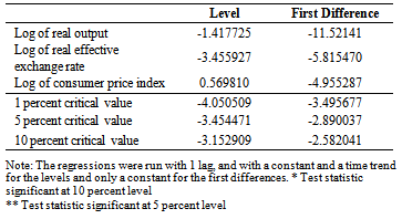
Estimation of the VAR model requires that each of the variables entering the model is stationary. Series that are non-stationary should be transformed appropriately prior to estimation; otherwise finite-sample inferences may suffer serious distortions. Appendix 1 (Figures A1-A6) plots the three variables used in the VAR in levels and first differences. It is clear that all the three variables have trended over the period and it is therefore necessary to determine whether the variables are stationary around stochastic or deterministic trends. Following the general econometric techniques for unit roots testing, the standard Augmented Dickey Fuller (ADF) test is employed. As usual, the appropriate lag level applied in the unit root tests follows the Schwarz Information Criterion (SIC). In testing for a unit root, we consider the possibility of a linear trend in levels of the three variables. The ADF test statistics as shown in Table 1 indicate that the null hypothesis of a unit root (non-stationarity) cannot be rejected for all the three variables. We further used the Augmented Dickey Fuller tests for the first difference of the variables and realized all were stationary, meaning, all the variables are integrated of order one; that is, they have I(1) processes. On the basis of these results (Table 1), it would be appropriate to estimate a reduced form VAR of the variables in their first differences.

Table 1. Tests for Stationarity

5.2. Cointegration Tests

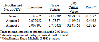
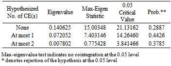
As pointed out by[19], even though individual time series are non-stationary, their liner combination might be stationary. When the linear combinations of non-stationary variables are stationary, the variables are said to be co-integrated. The technique makes it possible to test the existence of a long-term equilibrium among non-stationary variables. Though there is no economic reason to expect the variables in the model to be cointegrated, this is necessary to confirm the use of the VAR framework. If they are found to be co-integrated then the appropriate model will be a structural error correction model. To test this, we employ Johansen co-integration tests (see[20] and[21]). The results of the trace and maximum eigenvalues test statistics for the models are presented in Tables 2 and 3. Test results indicate that there is no evidence of cointegration among the three variables in consideration, hence a VAR in first differences is appropriate.

Table 2. Tests for Cointegration Rank Test (Trace)

Table 3. Tests for Cointegration Rank Test (Maximum Eigenvalue)

5.3. Granger Causality Analysis

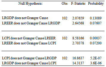
In order to get further insights into the dynamic interactions and the strength of causal relations among the different sources of real exchange rate fluctuations, the study proceeds with a Granger causality analysis. Basically, variable is said to be ‘Granger caused’ by variable if helps in the prediction of , that is, if the coefficients on the lagged are statistically significant at a given level. The directions of causality between the various sources of real exchange fluctuations signify important policy implications. For example, finding the direction of causality running from real GDP to real exchange rate means that real GDP may stimulate real exchange rate appreciations, which may in the end have consequences on the economy. Table 4 presents the pair-wise Granger causality tests between real GDP, real effective exchange rate and consumer price index. At 5% significance level we found significant causality for all pairs in both directions. In all cases we reject Ho that one of the variables not a Granger cause of the other. In other words real GDP and price levels Granger-causes real effective exchange rate. This is a good starting point for building the VAR model.

Table 4. Pairwise Granger Causality Tests

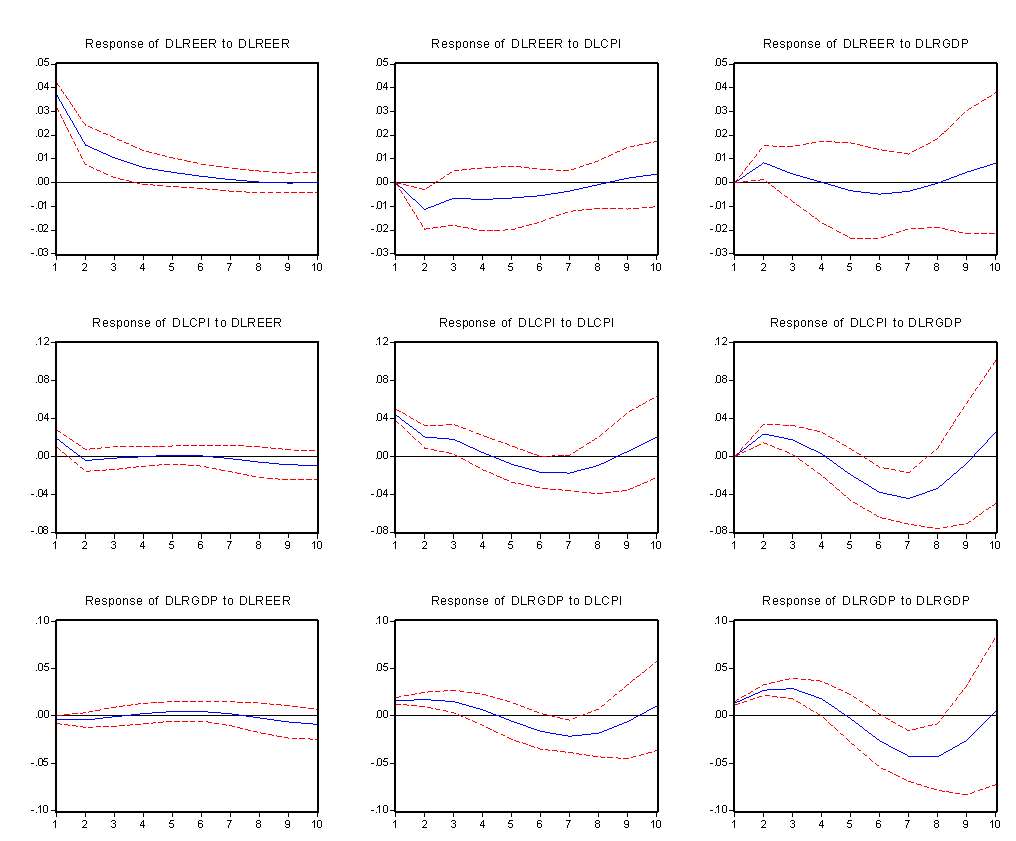Figure 2. Response to Cholesky One S.D. Innovations + 2 S.E

Table 5. VAR Granger Causality/Block Exogeneity Tests Equation Excluded Chi 2 Df Prob > chi 2 LREER LRGDP 5.843968 2 0.0538 LREER LCPI 18.81434 2 0.0001 LREER ALL 23.68745 4 0.0001

With regards to the VAR Granger Causality test (also known as the Block Exogeneity test), we test if the selected endogenous variables should not be treated as exogenous. The results as shown in table 5 strongly rejects the null hypothesis that variable excluded from the equation does not cause LREER. The results indicate that all variables in the model can be treated as endogenous (the remaining variables have significant impact on them jointly, but not always individually).

5.4. Impulse Response Functions

Having confirmed the existence of unit root and co-integration in the series and following the debates about advantages and drawbacks of different VAR specifications, we then proceed to estimate an unrestricted VAR system in first differences with two lags of each variable of the three equations. The paper by[22] demonstrated the advantages of unrestricted VAR by examining impulse response functions in cointegrated systems. Besides[18], other researchers like [23],[24] and[25] have shown the strengths of an unrestricted VAR is superior in terms of forecast variance. An intuitive way to interpret the variables in the VAR model is to compute an impulse response function (IRF) and Variance Decomposition measures. The impulse response function (IRF) traces out how the changes in one variable impact on current and future values of the endogenous variables in the model. The impulse response functions can be used to produce the time path of the dependent variables in the VAR, to shocks from all the explanatory variables. If the system of equations is stable, any shock should decline to zero. This also means that short-run values of the variable in question converge to the long-run equilibrium values. An unstable system would produce an explosive time path. In that sense, short-run values of the variable will diverge from its equilibrium values. Figure 2 displays the impulse response functions of the log of first differences of the variables (real exchange rate, consumer price index and real GDP) to one standard deviation structural shocks. The combined graphs are based on the output of the unrestricted VAR with analytic response standard error over 10 periods and Cholesky degrees of freedom adjusted, which show the response to Chelosky one standard deviation innovation. Each graph as shown in plots in Figure 2 includes a point estimation of impulse response functions as well as lower and upper bounds for a 95% confidence interval. As usual, the solid lines depict the variable percent change in response to a standard deviation of one in the respective macro variable whereas the dotted lines represent the 95% error bands.

The graph shows that the response of real effective exchange rate to its own shocks is contemporaneously strong and positive for the initial periods before it subsides to zero towards the end of the period. This means that any unanticipated increase in the real effective exchange rate consistently reduces the deviation between the short-term equilibrium values of the real effective exchange rate level and its long-run equilibrium values. The response of LREER to an unexpected shock to consumer price index is consistent but less persistent over the time horizons. It starts first by causing the deviation between the short-run equilibrium values of real effective exchange rate to decline after an unanticipated increase in consumer prices. However, the real effective exchange rate when disturbed by a shock in consumer prices could be stabilized only after the eighth quarter. Thereafter, it stabilizes and remains permanent. The impulse response functions for consumer prices and real GDP as a result of unanticipated shocks are also shown in the figure 2. Finally, an unexpected shock to LRGDP also has a predictable and stable relationship with real effective exchange rate. As can be observed from the graph, the impact of the shock will first cause LREER to increase (appreciate) up to 2^nd quarter and thereafter wanes and tends to decrease (depreciate) till the 7^th quarter is reached. Ultimately, the disturbance by a shock in real GDP is stabilized in the 10^th quarter. This is also consistent with the positive supply-side effect which causes prices on non-tradables to all and leads to the depreciation of the local currency.

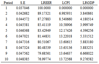
5.5. Variance Decomposition

Table 6. Variance Decomposition of LREER: VAR, 1986-2011 (in percent of total variance)

While impulse response functions trace the effects of a shock to one endogenous variable on other variables in the VAR, the alternative variance decomposition technique measures the proportion of forecast error variance in one variable explained by innovations in itself and the other variables. Thus, from the VDC, we can measure the relative importance of fluctuation of say, nominal or real shocks to variations in real exchange rate. To identify orthogonalised innovations in each of the variables and the dynamic responses to such innovations, variance-covariance matrix of the VAR was factorized using the Choleski decomposition method suggested by[26]. The results of the forecast error variance decomposition of the endogenous variables, at various quarters, generated by the three-variable, reduced form VAR model are shown in table 6.

Usually own series shocks explain most of the error variance, although the shock will also affect other variables in the system. As expected, the results show that the percentage of variance explained by own shock for real exchange rates declines to about 89 percent in the second quarter and continues falling until it ends with an average of around 77 percent at the end of the 10^th period. This indicates that real exchange rate is highly endogenous with the remaining factors accounting for the volatility in real exchange rate to varying degrees. The VDC demonstrate the significant role played by the nominal variables. For example, at the second quarter, the fraction of real exchange rates forecast error variance attributable to variations in consumer prices is about 7.0 percent. It then increases from the third quarter up to about 12.1 percent and by the end of the 10^th quarter, the contribution averages around 13.7 percent. The variance of real GDP accounts for about 3.8 percent in the second quarter, increases to about 4.4 percent in the 5^th quarter and increases further in the long term with an average value of 9.3 percent. It is also important to consider the ordering of the variables when conducting these tests, as in practice the error terms of the equations in the VAR will be correlated, so the result will be dependent on the order in which the equations are estimated in the model. The results did not significantly change with different ordering for the variables in the model. The overall findings confirm the importance of nominal variables in contributing to real exchange rate fluctuations in Ghana.

6. Conclusions and Policy Implications

Based on the assumption that there are several channels through which the exchange rate fluctuations can be perpetuated and that the ultimate effect on the economy may be muted or lessened depending on the actions or inactions of the fiscal and monetary authorities, this study employs the VAR methodology based on quarterly data for Ghana from 1986 to 2011 to analyze the relative importance of consumer prices and supply side shocks for fluctuations in the real effective exchange rate. The study has been able to establish Granger-causal relationships between real effective exchange rate and its fundamentals. Both supply and nominal shocks are very important in cushioning the real exchange rates against the appreciation in order to minimize the conventional Dutch Disease effects. The results show that consumer price increases (nominal shocks) contribute significantly to real effective exchange rate appreciations in Ghana. Policy should therefore be aimed at using additional inflows (such as additional oil revenues from new discovery) in Ghana to boost domestic production of tradable which would maintain higher export volumes. Additional resources should particularly be spent on a variety of investment goods such as machinery, spare parts and raw materials. The implementation of export friendly policies by government should also prove effective in moderating inflationary pressures induced by the additional inflows. It should be noted that this model serves only to indicate a possible equilibrium level based on the given economic fundamentals.

Appendix 1: Time Series Plots (Figure A1 – A6)

Figure A1. Time-Series Plot of log of Real Effective Exchange Rate (Levels)

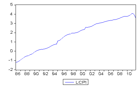Figure A2. Time-Series Plot of logs of Consumer Price Index (in levels)

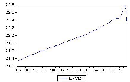Figure A3. Time-Series Plot of log of Real GDP (in Levels)

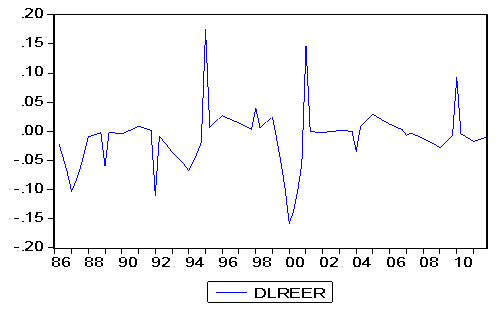Figure A4. Time-Series Plot of Real Effective Exchange Rate (First Differences)

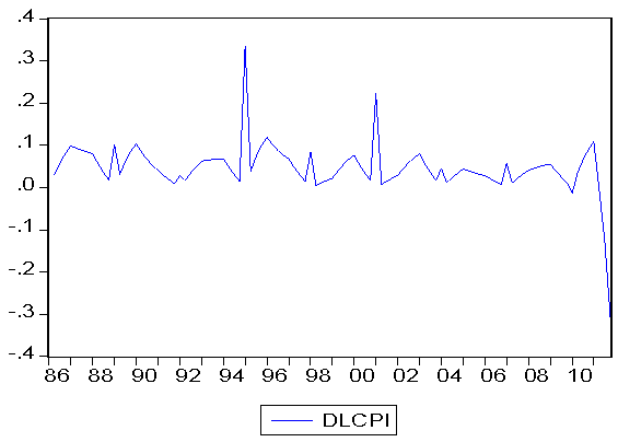Figure A5. Time-Series Plot Consumer Price Index (in first differences)

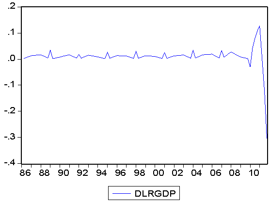Figure A6. Time-Series Plot of Real GDP (in first differences)

Appendix 2: Studies on the sources of real exchange rate fluctuations (RERF)

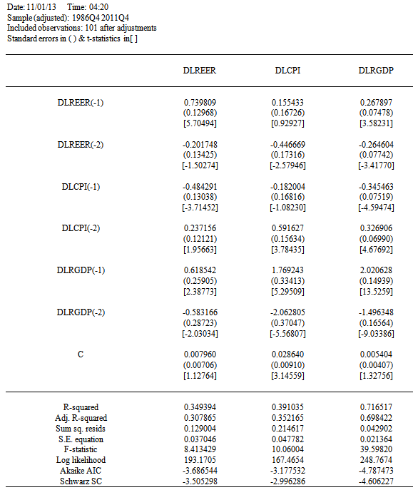
Appendix 3: Vector Autoregression Estimates

Notes

1. A summary of some of the studies on the sources of real exchange rate has been summarized in appendix 1.

2. Prominent studies that have tried to investigate the sources of real exchange rates fluctuations are summarized in the appendix.