M Monimul Huq1, M Mostafizur Rahman2, M Sayedur Rahman1, Md. Abu Shahin1, Md. Ayub Ali1
1Department of Statistics, University of Rajshahi, Rajshahi, 6205, Bangladesh
2Statistics and Mathematics School, Yunnan University of Finance and Economics, Kunming, 650221, China
Correspondence to: M Mostafizur Rahman, Statistics and Mathematics School, Yunnan University of Finance and Economics, Kunming, 650221, China.
| Email: |  |
Copyright © 2012 Scientific & Academic Publishing. All Rights Reserved.
Abstract
The purpose of the present study is to empirically examine the performance of different kinds of volatility modeling and their forecasting performance for the general index of an emerging stock market, namely Dhaka Stock Exchange from the period December 06, 2010 to March 12, 2013. We mainly used Box-Jenkins modeling strategy thereafter the volatility model. The descriptive statistics, correlogram, unit root test, ARMA, ARCH, GARCH, TARCH, EGARCH and several model selection criteria are used in this study. The Butterworth filter is used for removing the noise of the return series of general index. All the parameters in this study are estimated through Maximum Likelihood method. The descriptive statistics show general index decrease slightly overtime with positively skewed and leptokurtic. The return series follows ARMA(1,1) model with volatility provide evidence of the superiority of GARCH(1,1) and GARCH(2,1) over the all order of other GARCH models. Finally, we found that the fitted model on filtered general index of Dhaka Stock Exchange are ARMA(1,1) with GARCH(1, 1) and GARCH(2,1) model. This model can be used for future policy implication through its accurate forecast.
Keywords:
Butterworth Filter, Return Series, Unit Root, ARMA, GARCH, TARCH, EGARCH, Model Selection Criteria
Cite this paper: M Monimul Huq, M Mostafizur Rahman, M Sayedur Rahman, Md. Abu Shahin, Md. Ayub Ali, Analysis of Volatility and Forecasting General Index of Dhaka Stock Exchange, American Journal of Economics, Vol. 3 No. 5, 2013, pp. 229-242. doi: 10.5923/j.economics.20130305.04.
1. Introduction
Traditional regression tools have shown their limitation in the modeling of high-frequency data, assuming that only the mean response could be changing with covariates while the variance remains constant over time often revealed to be an unrealistic assumption in practice. This fact is particularly obvious in series of financial data where cluster of volatility can be detected visually. Indeed, it is now widely accepted that high frequency financial returns are heteroskedastic.Volatility is understood as the spread of asset returns and is closely related to risk. Volatility has pronounced role in modern finance as it is used in multiple risk management solutions. Volatility is the most important variable in valuating derivative instruments. It has central role in risk management, asset valuation and investment in general. Most stocks are traded on exchange, which are places where buyers and sellers meet and decide on a price. Bangladesh has two Stock Exchanges, Dhaka Stock Exchange (DSE) and Chittagong Stock Exchange (CSE), and these exchanges are self-controlled, private sector bodies which are obliged to get their functioning policies accepted by the SEC. Dhaka Stock Exchange (DSE) is the major stock exchange of Bangladesh and founded at Motijheel at the center of the Dhaka town in 1954 where buying and selling is carried out by Computerized Automated Trading System. Stock market volatility has been the subject of many studies over the past few decades. The main impetus for this interest began after the 1987 stock market crash where, for example, the Standard & Poor’s (S&P) composite portfolio dropped from 282.70 to 224.84 (20.4 %) and the Dow-Jones Average fell by 508 points in one day. The term stock market volatility refers to the characteristic of the stock market to rise or fall sharply in price within a short-term period (from day to day or week to week). Generally, increased volatility has been viewed as an undesirable consequence of destabilizing market forces such as speculative activity, noise trading or feedback trading. Increased volatility could come as a result of an innovation, by reflecting the actual variability of information regarding fundamental values. So an increased volatility may not necessarily be undesirable, Bollerslev et al[2].On the other hand policymakers may pursue regulatory reforms by either trying to reduce volatility directly or by assisting financial markets and institutions to adapt to increased volatility. In practice policy makers have focused on the latter, improving the ability of financial markets and institutions to weather increased volatility. For financial institutions directly exposed to increased volatility, such as depository institutions and market makers, policymakers have encouraged greater capitalization. Increased capital allows these institutions to weather greater financial volatility without incurring the liquidity and solvency problems that might disrupt the functioning of financial markets.The topic of volatility is of significant importance to anyone involved in the financial markets. In general volatility has been associated with risk, and high volatility is thought of as a symptom of market disruption, with securities unfairly priced and the malfunctioning of the market as whole. Especially, within the derivative security market volatility and volatility forecasting is vital as managing the exposure of investment portfolios is crucial, Figlewski[7]. More recently the literature has focused on the ability to forecast volatility of asset returns. There are many reasons why forecasting volatility is important according to Walsh and Yu-Gen Tsou[18], for example, option pricing has traditionally suffered without accurate volatility forecasts. Controlling for estimation error in portfolios constructed to minimize ex ante risk, with accurate forecasts we have the ability to take advantage of the correlation structure between assets. Finally when building and understanding asset pricing models we must take into account the nature of volatility and its ability to be forecasted, since risk preferences will be based on market assessment of volatility.There are many researchers analysis the share price index and they have noted that ARIMA with GARCH model is adequate. The average daily share price indices of the data series of Square Pharmaceuticals Limited (SPL) have been used and found that it is non-stationary at level, even after log-transformation, finally found that the ARIMA (2,1,2) is the best model (Paul et al.,[12]). The relationship between the stock market volatility and volatility in macroeconomic variables such as the real GDP, inflation, and interest rate are examine and found that there was a bi-directional causal relationship between stock market volatility and real GDP, and the stock prices were not significant in explaining the inflation rate and interest rate, and vice versa (Oseni and Nwosa,[11]). The analysis of daily return of Dhaka Stock Market indices include the daily price indices of all securities listed on the DSE general, DSI (All Share), DSE top 20 indices, and Daily indices listed in the market during the past 11 years and showed that DSE does not follow the random walk model and so the Dhaka stock exchange (DSE) is not efficient even in weak form (Khandoker et al.[9]). The data set of monthly DSE General Index (DSE-GEN) which covers the twenty three year long period commencing from January, 1987 to March, 2010 showed that it is follows random walk model but return series is not and the monthly DSE returns follow Generalized Autoregressive conditional Heteroskedasticity (GARCH) properties (Rayhan et al.[17]). Rahman et al[15] examined a wide variety of popular volatility models with normal, Student-t and GED distributional assumption for Chittagong Stock Exchange (CSE) and found that Random Walk GARCH (RW-GARCH), Random Walk Threshold GARCH (RW-TGARCH), Random Walk Exponential GARCH (RW-EGARCH) and Random Walk Asymmetric Power ARCH (RW-APARCH) models under Student- distributional assumptions are suitable for CSE. Rahman et al[16] investigated the in-sample and out-of-sample forecasting performance of GARCH, EGARCH and APARCH models under fat tail and skewed distributions in case of Dhaka Stock Exchange (DSE) from the period January 02, 1999 to December 29, 2005. From the above discussion it seems that volatility is important, since it directly and indirectly affects the financial system and the economy as a whole. The main aim of this research is to find out the appropriate model for the general index of Dhaka Stock Exchange (DSE). A further insight into volatility forecasting will be given but first it is necessary to explore the different models used when estimating volatility. Therefore, the Objective of this Study is to compare the performance of different kind of volatility modeling and to establish the forecasting efficiency of the fitted model in case of DSE. Rest of the paper is organized as follows: Section 2 presents the method and materials, Section 3 discuss the empirical results and finally Section 4 presents the conclusion.
2. Methods and Materials
We consider daily stock exchange data (general index) for building time series modeling and forecast. To fulfill this purpose we collect data from the databank of the Dhaka Stock Exchange website addresswww.dsebd.org/recent_market_information.php. The data series is from December 06, 2010 to March 12, 2013 and the length is 541. In analyzing general index data, the general index must be converting as return series because it is seen as the white noise process which indicates that index price is a random walk, the series should be identically and independently distributed with zero mean and constant variance (Akgiray,[1]). A white noise suggests that the future values of the expected mean and variance of the series cannot be predicted by using past values of the series. The return series are constructed using DSE general index to allow a market wide measure of volatility to be examined. By convention, the daily returns were calculated as the continuously compounded returns which are the first difference in logarithm of closing prices of DSE general index of successive days: Generally, the return series (or general index) is random but it is widely affected by the noise. Since the main purpose of modeling for general index is to find out actual nature hence we can apply different filtering for removing noise. There are several filter method are available but we only consider Butterworth filter in this study. The Butterworth filter proposed by British engineer Stephen Butterworth in his paper entitled "On the Theory of Filter Amplifiers” at 1930 is a type of signal processing filter designed to have as flat a frequency response as possible in the pass band.Let us consider a time series
  for considered as filtering. We are interested in isolation component of
  , denoted
  with period of oscillations between
  and
and  , where
  .Consider the following decomposition of the time series
 The component
  is assumed to have power only in the frequencies in the interval
  .
.  and
and  are related to
 and
and  by
by If infinite amount of data is available, then we can use the ideal band pass filter
  where the filter,
  , is given in terms of the lag operator L and defined as
 The ideal band pass filter weights are given by
 The digital version of the Butterworth high pass filter is described by the rational polynomial expression (the filter’s z-transform)
 The time domain version can be obtained by substituting z for the lag operator L.Pollock derives a specialized finite-sample version of the Butterworth filter on the basis of signal extraction theory. Let
  be the trend and
  cyclical component of
  , then these components are extracted as
 where
where  and
and  If we consider drift is true, then the drift adjusted series is obtained as
 where
where  is the undrafted series.The software Microsoft Excel, Eviews, R and Microsoft Word are used whole analysis and written in this paper.
2.1. Autoregressive Moving Average (ARMA) Process
Of course, it is quite likely that a time series has characteristic of both AR and MA and is therefore ARMA. An ARMA process of order p and q is denoted by ARMA(p, q) and is written in the form: | (1) |
Where  are AR and MA coefficients, respectively, and,
  white noise disturbance terms.In general the ARMA (p, q) process can be written as a stationary ARMA process has the following form of theoretical ACF and PACF;v The theoretical ACF decays,v The theoretical PACF are also decays.
2.2. Autoregressive Conditional Heteroscedastic (ARCH) Model
Let us consider a univariate time series  . If
. If  is the information set (i.e. all the information available) at time
 , we can define its functional form as:
 | (2) |
where  denotes the conditional expectation operator and
  is the disturbance term (or unpredictable part), with
  The
The  term in equation (2) is the innovation of the process. The conditional expectation is the expectation conditional to all past information available at time
  . The Autoregressive Conditional Heteroscedastic (ARCH) process of Engle[5] is any
  of the form
 | (3) |
where  is an independently and identically distributed (i.i.d.) process,
  is a time-varying, positive and measurable function of the information set at time
  . By definition,
  is serially uncorrelated with mean zero, but its conditional variance equals to
  and, therefore, may change over time, contrary to what is assumed in OLS estimations. Specifically, the ARCH (q) model is given by
 | (4) |
The models considered in this paper are all ARCH-type. They differ on the functional form of  but the basic logic is the same.
2.3. Generalized ARCH (GARCH) Model
Engle used the conditional variance to be autoregressive. Bollerslev[2] extended Engle’s ARCH to include the lagged variance according to ARMA process. Bollerslev’s generalized autoregressive conditional heteroskedastic process take the following form. The error process is given by | (5) |
Using the lag or backshift operator  , the GARCH (p, q) model is
 | (6) |
with  and
and  based on equation (6), it is straightforward to show that the GARCH model is based on an infinite ARCH specification. If all the roots of the polynomial
  of equation (6) lie outside the unit circle, we have
 or equivalently
  which may be seen as an ARCH(
 ) process since the conditional variance linearly depends on all previous squared residuals. GARCH(1,1) model can be obtain from equation (5) by using the value
  .
.
2.4. Threshold GARCH (TARCH) Model
TARCH or Threshold ARCH and Threshold GARCH were introduced independently by Zakoïan[19] and Glosten, et al[6]. The generalized specification for the conditional variance is given by: | (7) |
where  In this model
  have differential effects on the conditional variance;
  has an impact of
  , while
  has an impact of
  . If
. If  increases volatility, and we say that there is a leverage effect for the
  the news impact is asymmetric.
2.5. Exponential GARCH(EGARCH) Model
The EGARCH or Exponential GARCH model was proposed by Nelson[10]. The specification for conditional variance is: | (8) |
The left hand side of equation (8) is the log of the conditional variance. This implies that the leverage effect is exponential rather than quadratic and that forecasts of the conditional variance are guaranteed to be non-negative. The presence of the leverage effects can be tested by the hypothesis  . The impact asymmetric if
  .
.
3. Results and Discussions
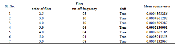
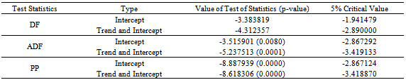
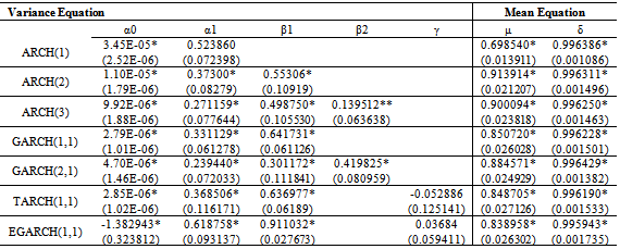
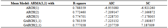
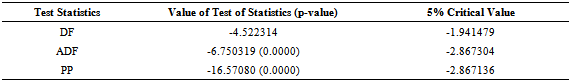
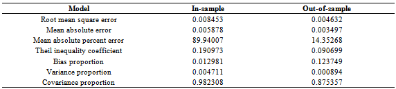
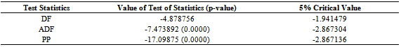
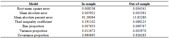
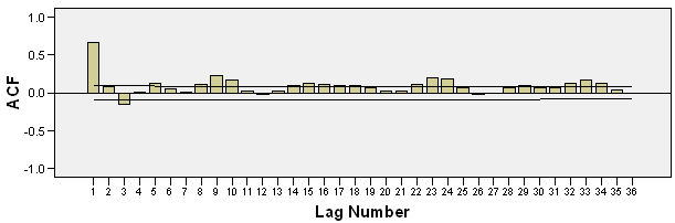
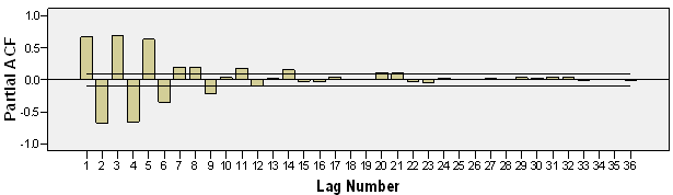
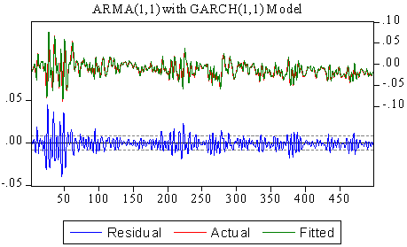
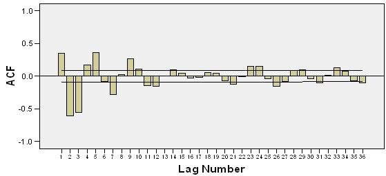
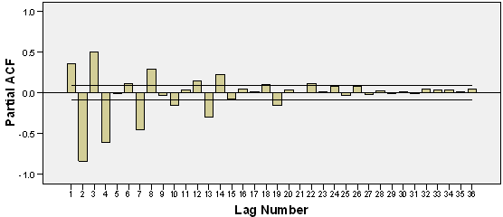
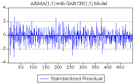
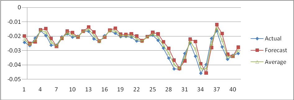
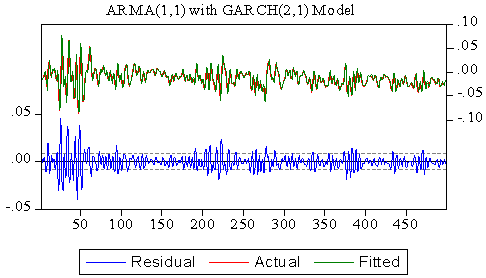
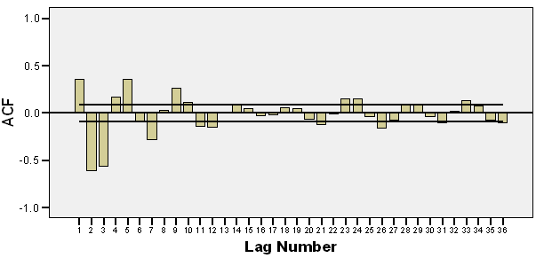
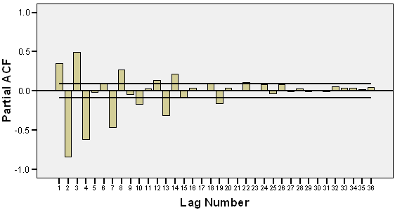
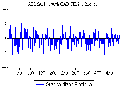
We collect data of general index from Dhaka Stock Exchange, Bangladesh from December 06, 2010 to March 12, 2013 with 541 realizations. We divided sample into two parts such as first 499 and last 42 samples for training and test sample, respectively to permit more efficient model. The most popular programming software R and econometrical software Eviews used to whole analysis according to objective of present research. Throughout this paper, the general index is converted into stock returns are defined continuously computed or log returns (hereafter returns) at time because it is more stable then original general index. It has been observed that the return series as well as general index is very much affected by noise. So the actual behavior of the series is hidden by noise and hence we cannot meet to the main objective of analysis. Therefore, we can remove the noise from return series using filtered methods. There are many methods are available for filtering of a time series, in this case we consider Butterworth high pass filter but this filter is very much affected by different values of order of filter and cut-off frequency. So, we consider different values of order of filter and cut-off frequency for filtering return series and finally chose the filtered series if it gives smallest mean square error. The different values of order of filter and cut-off frequency with mean square error are presented in Table 1. From Table 1, it is clear that the filtered series for 3rd order filter with cut-off frequency is 4 (Sl. No. 4) gives smallest MSE (mean square error) as considered de-noise actual study series. From the selected filtered return series (Sl. No. 4 in Table 1), the trend indicated by red color (top of Figure 1) is used as study series; cyclical component is ignored and indicates noise of original return series. We observed that the deviations (cyclical component) are very small. In the next, we will be used this filtered return series (trend) for fulfill according to our objectives. The Table 2 reports summary statistics for the filtered return series of general index. The mean and median of daily returns are negative and they are not significantly different from zero. It suggests that stock prices in general decrease slightly overtime. The skewness and kurtosis parameters respectively measure the asymmetry and peakness of the probability distribution of filtered daily returns compared with normal curve usually these two parameters should be zero and three in normal distribution. The Jarque-Bera statistic with skewness and kurtosis are used to signify the distribution characteristics of return series. In the data set, the evidence for return series indicates positively skewness of daily return distribution. In other words, return series distribution has significantly fatter tails than the normal distribution. The coefficient of skewness indicates that the series typically have asymmetric distributions skewed to the right. The kurtosis statistic which is equal to 5.52 indicates the leptokurtic characteristic of the daily return distribution. The return distribution has a more acute peak around the mean than the normal distribution. The implication of non-normality is supported by the Jarque-Bera test statistic which points out that the null hypothesis of normal distribution is rejected. In accordance with the skewness and kurtosis, the Jarque-Bera statistic is another evidence to conclude that the daily return series is not normally distributed. Also from the filtered return series indicates that the series variance is not constant over time suggests that models employed need to take into account heteroskedaticity issues, indicating the reasonable use of GARCH type models (Bollerslev,[2]).Researchers are interested in the first step of the analysis of any time series is to plot the data to see the visual structure. Time series plot gives an initial clue about the nature of the series or shows an upward or downward trend, seasonal or cyclical fluctuation etc. Graphical representation suggests that the time series is stationary or not. The filtered return series (red color named trend located top of Figure 1) shows that the mean returns is constant but the variances change over time around some normal level, with large (small) changes tending to be followed by large (small) changes of either sign, i.e. volatility tends to cluster. Periods of high volatility can be distinguished from low volatility periods. Now ACF and PACF of the filtered series are plotted in Figure 2 and 3, and see almost all of the coefficients of ACF and PACF inside the confidence limits. Again the ACF converge to zero very quickly, which indicated that the series is stationary.Finally, unit root test is used to confirm the series is stationary or not. The unit root test results for filtered return series are shown in Table 3. The Table 3 showed different unit root test with p-values and critical values for filtered return series of general index of DSE. The results of Dickey-Fuller (DF), Augmented Dickey-Fuller (ADF) and Phillips-Perron (PP) tests showed that the filtered series data is stationary. So we can say form graphical representation, correlogram and unit root test the filtered data series is stationary. We now proceed to build models. Now we can build ARMA Model using the filtered daily return series because it is stationary at level. Using the Box-Jenkins modeling strategy the model ARMA(1,1) is better among the various combinations of model parameters p and q of ARMA(p,q). Now we want to test whether the heteroskedaticity problem is exist or not and that is permit using more formal Lagrange multiplier test for ARCH disturbances proposed by Engle[5]. The calculate value of test statistics (F-value) of Lagrange multiplier test up to lag 4 is 80.08300 with probability 0.00000 indicates the presence of ARCH effect in the residual series of ARMA(1,1) model.Therefore, we have to search the family of GARCH type Models. We simultaneously model the mean and the variance of Dhaka Stock Exchange, considering the ARCH, GARCH, TARCH and EGARCH models for conditional variance. Table 4 present the results from seven alternative models including ARCH(1), ARCH(2), ARCH(3), GARCH (1,1), GARCH(2,1), TARCH(1,1) and EGARCH(1,1) employed in this dissertation to estimate volatility for the period from December 06, 2010 to January 10, 2013 in Dhaka stock Exchange. We already saw that in our data the heteroskedastic problem is present. Thus the ARCH class models may give the better result. Now we apply the various ARCH models under the assumption of normal distribution for return data which gives the results shown in Table 4. At first we examined symmetric ARCH (1) model. This specification gives that the coefficient of ARCH(1) model is significant in parameters. Also mean equation with ARMA(1,1) model parameters are also significant. We also observed ARCH(2), ARCH(3) models where all the parameters also significant. But ARCH(4) and higher order model parameters are insignificant.We also perform a higher order of GARCH estimation allowing the ARCH and GARCH term to enter the variance equation with more than one lags. Therefore, we then carry out the GARCH(1,q) model allowing more lags of GARCH terms involved in volatility equation. The coefficients in variance equation estimated from GARCH(1,1) and GARCH(2,1) models are positive and highly statistically significant. However, when the higher order of GARCH terms are added into the variance equation, the statistics of the new GARCH term is less significant or it makes the other terms’ statistic less significant. Thus result suggests that GARCH(1,1) and GARCH(2,1) models are sufficient enough to capture volatility characteristics of Dhaka Stock market without the need of higher-order GARCH models. The skewness statistics of the return series which are generated in Table 2 and Table 2 imply the asymmetry in the data set. Therefore, the asymmetric specifications of GARCH model, TARCH and EGARCH, are also employed in this dissertation. However, regarding the results of those asymmetric models, the so-called asymmetric effect parameter γ is not statistically significant at 10% and 5% level for TARCH and EGARCH, respectively. Though, the coefficient of mean equation in both models is significant at 1% level. This implies the weak evidence of asymmetry in the return series. In other words, the conditional variance is not higher in the presence of negative innovation or the market seems not nervous when bad news takes place. The finding is interesting because it is likely a phenomenon in many mature markets that the investors react more dramatically to negative shocks than positive shocks. However, the outcome is consistent with the findings in some other emerging markets such as transition markets of Central Europe (Haroutounian and Price,[8]).According to Chou[3], the sum of ARCH and GARCH terms’ coefficients α1 + β1 present the change in the response function of shocks to conditional variance per period. Poterba and Summber[14] showed that the impact of the volatility on stock prices crucially depends on the persistence of shocks to variance over a long time. The parameters from Table 4 point out that the sum of α1 and β1 is close to unity across the two models including GARCH(1,1), GARCH(2,1) models. The high persistence of shock to variance is supported by previous studies in the case of emerging capital markets. The finding implies that available information is relevant in forecasting conditional variance at long time horizon.Generally, coefficients in variance equation obtained from two estimation models including GARCH(1,1), GARCH(2,1) are highly statistically significant at 1% level. Moreover, the higher order GARCH (p,q) models generate the insignificant parameters, indicating the sufficiency of GARCH(1,1) and GARCH(2,1) in modelling volatility of Dhaka stock index returns. Meanwhile, the findings from TARCH and EGARCH provide weak evidence of asymmetry in return series, which is consistent with empirical studies in some emerging markets. In Table 5 we examined R-square value, Akaike Information Criterion (AIC) and Schwartz -Criterion (SC) from different models. From Table 5 we found that the value of R-square, AIC and BIC of GARCH(1,1) and GARCH(2,1) are almost equal and smallest of all other models. So, we can proceeds these two models for further analysis of diagnostic check and forecasting. Firstly, we can consider ARMA(1,1) with GARCH(1,1) model for diagnostic checking and forecasting. The graphical presentation of this fitted model is helpful for inspection the performance of fitted model and presented as Figure 4. We observed from Figure 4 which is the plot of residual, actual and fitted model data and conclude that the GARCH(1,1) model is fit well. Model diagnostic checking is an important step for selecting an appropriate model. Usually residual analysis is the best way for model checking. Now we shall observe the correlogram, unit root test of residual to check it is stationary or not. In order to check the white noise property of the estimated ARMA(1,1) with GARCH(1,1) model residual, we constructed ACF and PACF of the residual series presented by Figure 5 and 6. From Figure 5 and 6, the ACF and PACF tapper of very quickly, this implies that the residual series is stationary. Then we can say that the model is appropriate. The Table 6 showed different unit root test with p-values and critical values for residual of ARMA(1,1) with GARCH(1,1) model. The results of Dickey-Fuller (DF), Augmented Dickey-Fuller (ADF) and Phillips-Perron (PP) tests showed that the residual is stationary. So we can say that the assumption of chosen model is appropriate.To test of ARCH effect in the residual series of fitted the ARMA(1,1) with GARCH(1,1) model, we can consider Lagrange multiplier (LM) test of the residuals. We observed that the calculated value of F statistic for Lagrange multiplier test is 0.543470 with associated probability is 0.461348 indicating no ARCH effect in residuals of ARMA(1,1) with GARCH(1,1) model. Therefore, the chosen model for volatility may be adequate. The properties of standardized residuals are employed to define the best fit data models. Standardized residual plot is a very useful tool to check the presence of unusual observations. Standardized residual from the model in presented in Figure 7 has some positive and some negative values that falls in three standard deviation confidence interval except one. But it falls in four standard deviation confidence interval. This is the strong indication that the ARMA(1,1) with GARCH(1,1) model is appropriate. The test of normality in this study we used Jarque-Bera test. We observed that the calculate value of Jarque-Bera test is 0.533484 with Probability 0.765870 indicate the null hypothesis ‘The residual series of fitted model is normal’ is accepted. Therefore, the estimated residuals of the fitted ARMA(1,1) with GARCH(1,1) model is normally distributed.A forecast is generally defined as a statement concerning future events. Forecasting is one of the most common uses of econometric methods. According to Akgiray[1], there are two reasons why forecasting volatility attracts interests of investors. Firstly, good forecast capability of volatility models provides a practical tool for stock market analysis. Secondly, as proxy for risk, volatility is related to expected returns, hence good forecast models enable investors give more appropriate securities pricing strategies. However, in-sample and out-of-sample forecast evaluation potentially provides more useful comparison. Now we will cheek the adequacy of the fitted model using the in-sample and out-of-sample, root mean square error, mean absolute error, mean absolute percent error, Theil inequality coefficient, bias proportion, variance proportion and covariance proportion of forecast properties. If the in-sample root mean square error, mean absolute error, mean absolute percent error, Theil inequality coefficient, bias proportion, variance proportion and covariance proportion are greater than the out-sample with same criteria then this fitted model is adequate. We have used all data from 12/05/2010 to 01/10/2013 (sample size 499) as the ‘in-sample’ period and the out sample data from 01/13/2013 to 03/12/2013 (last sample size 42) as the ‘out-of-sample’ period. Now the calculated values of forecast properties for in sample and out sample are presented in Table 7. From Table 7, the values of root mean square error, mean absolute error, mean absolute percent error, Theil inequality coefficient, variance proportion and covariance proportion for in sample is greater than for out sample implies that the selected model is adequate. The bias proportion for in sample is less than out sample that is unexpected but that is occurs because the out sample size is very smaller compared with in sample. Therefore we can say on the basis of forecast properties the selected model ARMA(1,1) with GARCH(1,1) is adequate. Thus, the forecasting performance of selected model can be represented by graphically as Figure 8. The Figure 8 shows the actual filtered series, forecasted series and their average for the period 01/13/2013 to 03/12/2013. It is evident from Figure 8, forecast values, observed values and average values are very close to each other. So the model ARMA(1,1) with GARCH(1, 1) forecasting performance is reasonable. Secondly, we can consider ARMA(1,1) with GARCH(2,1) model for diagnostic checking and forecasting. We can explain the ARMA(1,1) with GARCH(2,1) model similar way of the ARMA(1,1) with GARCH(1,1) model. The graphical presentation of this fitted model represented as Figure 9. The fitted model ARMA(1,1) with GARCH(2,1) (Figure 9) shows the actual and fitted values of return series is very close and the error is very small indicating model is fit well. Now, we shall need to check the estimated residual is stationary or not. We can check stationarity of the residual series using autocorrelation and partial autocorrelation function and unit root test. The autocorrelation and partial autocorrelation function of residual series of ARMA(1,1) with GARCH(2,1) model presented in Figure 10 and 11. We observed the Figure 10 and 11, the spikes of autocorrelation and partial autocorrelation function are converse to zero very quickly imply the residual series is stationary. To conform the residual series of ARMA(1,1) with GARCH(2,1) model is stationary, we used the formal test of stationary Dickey Fuller (DF), Augmented Dickey Fuller (ADF) and Phillips Perron (PP) tests are presented in Table 8. The null hypothesis ‘The residual series contain unit root’ is rejected for all test (DF, ADF and PP test) implies the residual series is stationary. We observed the return series of general index is contains volatility problems so we used the GARCH type of model for controlling volatility effect. So after such volatility modelling we must check whether their volatility effect exist or not. The Lagrange multiplier test is used for testing ARCH effect. The calculate value of test statistics (F-value) of Lagrange multiplier test with lag 1 is 0.357910 with probability 0.549943 imply the null hypothesis is accepted and it is evidence of the absent of ARCH effect in the ARMA(1,1) with GARCH(2,1) model of filtered return series. The standardized residual plot is used whether the data series contain the some specific values (usually ±3 standard deviation) otherwise consider as outliers. The standardized residual plot for ARMA(1,1) with GARCH(2,1) model is presented in Figure 12. From Figure 12, it is clear that the all standardized residuals are lies within (-3 to +3) except one. Hence, model is fitted well. The normality of residual series can be test using Jarque Bera test statistics. The null hypothesis of Jarque Bera test statistics is the residual series is normally distributed. The calculated vale of Jarque Bera test statistics is 1.231352 with probability 0.540276 indicating the null hypothesis is accepted that means the residual series of ARMA(1,1) with GARCH(2,1) model is normally distributed.Finally, we can check the model adequacy using various model selection criteria for in-sample and out-sample forecast of chosen model. The forecasting evaluation based on various forecasting error criteria of ARMA(1,1) with GARCH(2,1) model is summarized the in Table 9. We know that if the Root mean square error, mean absolute error, mean absolute percent error, Theil inequality coefficient, bias proportion, variance proportion and covariance proportion are smaller for out-sample forecast than in-sample forecast considered as best model. We observed the Table 9, the all value for Root mean square error, mean absolute error, mean absolute percent error, Theil inequality coefficient, variance proportion and covariance proportion are smaller for out-sample forecast than in-sample forecast but bias proportion is reverse. The bias proportion for in sample is less than out sample that is unexpected but that is occurs because the out sample size is very smaller compared with in sample. Hence we can say the chosen ARMA(1,1) with GARCH(2,1) model is adequate. The actual, forecast and average values for out-sample are presented as Figure 13 and indicates the difference between actual and forecast values are very small. Therefore, the chosen ARMA(1,1) with GARCH(2,1) model is acceptable.
4. Conclusions
The general index of stock market is very important index for the analysis and predicting investment. The general index of Dhaka Stock Market over the time 5 December 2010 to 10 January 2013 with sample size is 499 were used in this study. The preliminary analysis of data set suggests the non-normal distribution and strong evidence of GARCH effects in filtered general index return series. At the beginning of the study general index data of Dhaka Stock Exchange has been explored and analyzed using visual inspection of original data, return series that is also filtered by using Butterworth filter. The filtered return series has constant mean but the variance is not constant. To check the stationarity, we perform test of correlogram and unit root test which indicate that the return series is stationary. Then we construct several mean models as well as variance models. Both symmetric and asymmetric models used in this study and finally found that the model ARMA(1,1) with GARCH(1,1) and GARCH (2,1) are more appropriate model for the general index of Dhaka Stock Exchange (DSE) for this study period. This result will provide informative guide line for the researchers and policymaker.
ACKNOWLEDGEMENTS
This research was supported by Yunnan University of Finance and Economics.
Appendix A
Table 1. Butterworth filter with different order, cut-off, drift and mean square error
 |
| |
|
Table 2. Descriptive Statistics for daily return series of DSE General Index
 |
| |
|
Table 3. Unit root test of filtered return series
 |
| |
|
Table 4. Maximum Likelihood estimates of several ARCH, GARCH, TARCH and EGARCH models
 |
| |
|
Table 5. The following table gives R-square, AIC and SC of some different models
 |
| |
|
Table 6. ADF and PP test of the residual series of ARMA(1,1) with GARCH(1,1) model
 |
| |
|
Table 7. Results of in-sample and the out-of-sample forecast properties of fitted model
 |
| |
|
Table 8. Unit root test of residual series for ARMA(1,1) with GARCH(2,1) model
 |
| |
|
Table 9. Results of in-sample and the out-of-sample forecast properties of fitted model
 |
| |
|
Appendix-B
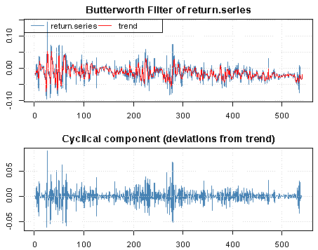 | Figure 1. Plot of Butterworth filter of return series of GI series and deviation from trend |
 | Figure 2. ACF of filtered return data of DSE |
 | Figure 3. PACF of filtered return data of DSE |
 | Figure 4. Actual, fitted and residual of ARMA(1,1) with GARCH(1,1) |
 | Figure 5. ACF of residual of ARMA(1,1) with GARCH(1,1) |
 | Figure 6. PACF of residual of ARMA(1,1) with GARCH(1,1) |
 | Figure 7. Standardized residual obtained from ARMA(1,1) with GARCH(1,1) model |
 | Figure 8. Forecast, observed and average values of out-of-sample forecast for ARMA(1,1) with GARCH(1,1) model |
 | Figure 9. Actual, fitted and residual graph for ARMA(1,1) with GARCH (2,1) model |
 | Figure 10. ACF of residual of ARMA(1,1) with GARCH(2,1) |
 | Figure 11. PACF of residual of ARMA(1,1) with GARCH(2,1) |
 | Figure 12. Standardized residual plot of ARMA(1,1) with GARCH(2,1) |
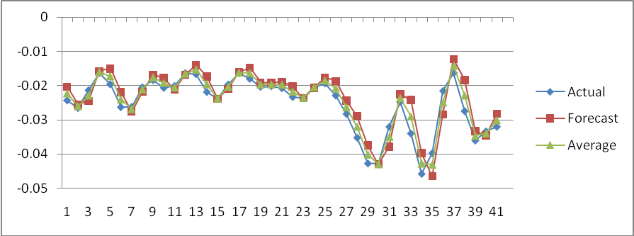 | Figure 13. Forecast of out of sample of ARMA(1,1) with GARCH(2,1) |
References
| [1] | Akgiray, V. 1989, Conditional heteroskedasticity in time series of stock returns: evidence and forecasts, Journal of Business, 62, 55-80. |
| [2] | Bollerslev, T., Chou, R. Y., and Kroner, K. F., 1992, ARCH modelling in Finance, Journal of Econometrics, Vol. 52, pp. 5-59. |
| [3] | Chou, R. 1988, Volatility persistence and stock valuation: Some empirical evidence using GARCH, Journal of Applied Econometrics, October/December 1988, 3, 279-294. |
| [4] | Dickey, D, A., Fuller, W. A. 1979, Distribution of the estimators for autoregressive time series with a unit root, Journal of the American statistical association, vol. 74, pp. 427–431. |
| [5] | Engle, R. F. 1982, Autoregressive conditional heteroscedasticity with estimates of the variance of United Kingdom inflation. Econometrica, 50,987-1007. |
| [6] | Glosten, L.,Jagannathan, R. and Runkle, D., 1993, On the relation between expected return on stocks, Journal of Finance, 48, 1779–1801. |
| [7] | Figlewski, S., 1997, Forecasting Volatility, Financial Markets, Institutions and Instruments, Vol. 6, Blackwell Publishers. (Note: final draft 2004) |
| [8] | Haroutounian M. K and Price, S. 2001, Volatility in the transition markets of Central Europe, Applied Financial Economics, 11, 93-105. |
| [9] | Khandoker, M.S.H., Siddik, M.N.A., Azam, M. 2011, Tests of Weak-form Market Efficiency of Dhaka Stock Exchange: Evidence from Bank Sector of Bangladesh. Interdisciplinary Journal of Research in Business. Vol. 1, Issue. 9, 47- 60. |
| [10] | Nelson D. 1991, Conditional heteroskedasticity in asset returns: a new approach, Econometrica, 59, 347-70. |
| [11] | Oseni, I.O., Nwosa, P.I., 2011, Stock Market Volatility and Macroeconomic Variables Volatility in Nigeria: An Exponential GARCH Approach. Journal of Economics and Sustainable Development. Vol.2, No.10, 2011. |
| [12] | Paul, J.C., Hoque, M.S., Rahman, M.M. 2013, Se lection of Best ARMA Model for Forecasting Average Daily Share Price Index of Pharmaceutical Companies in Bangladesh: A Case Study on Square Pharmaceutical Ltd. Global Journal of Management and Business Research Finance. Vol. 13 Iss. 3. |
| [13] | Phillips, P.C.B., Perron, P. 1988, Testing for a unit root in time series regression, Biometrika, vol. 75, pp. 335–346. |
| [14] | Poterba L. and Summbers L. 1986, The Persistence of Volatility and Stock Market Fluctuations American Economic Review, 76, 1142-1151. |
| [15] | Rahman, M. M., Zhu, J. P., and Rahman, M. S. 2008, Impact study of volatility modeling of Bangladesh stock index using non-normal density, Journal of Applied Statistics, Vol. 35, No. 11, 1277-1292. |
| [16] | Rahman, M. M., Huq, M.M and Rahman, M. S. 2012, In sample and out of sample forecasting performance under fat tail and skewed distribution. Proceeding book of International Conference on Statistical Data Mining for Bioinformatics, Health, Agricultural and Environment, 462-472. |
| [17] | Rayhan, M. A., Sarker, S.A.M.E., and Sayem, S.M. 2011, The Volatility of Dhaka Stock Exchange (DSE) Returns: Evidence and Implications. ASA University Review. Vol. 5 No. 2, July–December, 2011. |
| [18] | Walsh, D., M., and Yu-Gen Tsou, G., 1998, Forecasting index volatility: sampling interval and non-trading effects, Applied Financial Economics, Vol. 8, (5), pp. 477-485. |
| [19] | Zakoian, J. M. 1994, Threshold Heteroscedastic Models, Journal of Economic Dynamics and Control, 18, 931–955. |
 Abstract
 Reference
 Full-Text PDF
 Full-text HTML