-
Paper Information
- Previous Paper
- Paper Submission
-
Journal Information
- About This Journal
- Editorial Board
- Current Issue
- Archive
- Author Guidelines
- Contact Us
American Journal of Economics
p-ISSN: 2166-4951 e-ISSN: 2166-496X
2012; 2(6): 136-145
doi: 10.5923/j.economics.20120206.08
Distributions of Intergenerational Earnings: A Nonparametric Analysis of Racial Differences
 Abstract
 Reference
 Full-Text PDF
 Full-Text HTML
Darrell J. Glaser
Department of Economics, United States Naval Academy, 589 McNair Road, Annapolis, MD 21402-5030, USA
Correspondence to: Darrell J. Glaser , Department of Economics, United States Naval Academy, 589 McNair Road, Annapolis, MD 21402-5030, USA.
| Email: |  |
Copyright © 2012 Scientific & Academic Publishing. All Rights Reserved.
Nonparametric methods are used to analyze distributions of intergenerational earnings. A stochastic kernel generates stationary distributions for African-Americans and whites, indicating a long-run outcome not in favor of racial convergence. Tests indicate that the distribution of white earnings stochastically dominate the earnings distributions of African-Americans from similar economic backgrounds. Within-race decile comparisons demonstrate that the distributions for whites improve as fathers' earnings improve; each increase in fathers' deciles progressively improves the entire distribution for sons. The same results do not exist for African-Americans who appear to have extensive within-race mobility.
Keywords: Intergenerational Mobility, Earnings Inequality, Convergence, Non-Parametric Distributions
Article Outline
1. Introduction
- Explanations of whether or how children's economic outcomes follow those of their parents, such as attaining similar levels of education, moving into similar occupations, or ultimately achieving similar levels of income, have received extensive attention. Few studies, however, have analyzed differences in mobility between different populations, or the structure of distributional differences across races. The nonparametric methods used in this paper serve a useful role for analyzing small samples, as in the distributions pulled from the PSID, and they also provide elements of objectivity to ongoing discussions regarding the presence and structure of nonlinearities in intergenerational outcomes. Rather than arguing for or against a specific nonlinear functional relationship in the development ofintergenerational earnings, inference via nonparametric methods allows the data to speak for itself, without researcher imposed assumptions on intergenerational structure. To address this, research in this paper measuresdifferences in intergenerational earnings mobility ofAfrican-American and white sons across the entire distribution of fathers' economic outcomes and statistically tests between-race and within-race differences in the distribution of outcomes. In general, results indicate that African-American sons not only have lower conditional means than their white peers from similar economic backgrounds, but also that the distribution of outcomes for African-Americans repeatedly skews towards lower earnings than the outcomes of whites. The evidence suggests that African-Americans do worse than whites except among those born in the highest deciles. Furthermore, within-race comparisons of white earnings demonstrates the stochastic dominance of white sons whose fathers' earned in higher deciles over those whose fathers earned in successively lower deciles. The implication is that whites exhibit very little intergenerational mobility. This should not surprise us, since it appears to support what we already believe about slowing rates of convergence. In contrast to this, this same result does not exist for the distributions of African-Americans except for some deciles in the middle class. African-Americans in general show extensive within-race intergenerational mobility (i.e. convergence), a result that previous research in this field has not confirmed. Results throughout the paper indicate that earnings outcomes for the two races follow two distinctly different stochastic processes. While primarily descriptive in nature, the evidence is compelling enough to argue that simple point estimates of the degree of intergenerational convergence are incomplete and indeed often misleading.The remaining sections address related literature in section 2 and transition probabilities in section 3. Issues with regard to data, including measurement error corrections, follow in section 4. Section 5 includes the analysis of intergenerational distribution dynamics. These include discussions ofstationary distributions, the stochastic dominance ofdecile-conditioned white distributions over African-American distributions, and within-race comparisons of decile conditioned distributions. Section 6 provides a brief conclusion.
2. Related Literature
- Much of the empirical work on intergenerational mobility extends back to the seminal works of Sir Francis Galton[1] and[2], who hypothesized on the parental transmission of attributes such as schooling, height and earnings to children. The Galton framework of intergenerational mobility has historically estimated some form of the conditional mean. The methodology of regression analysis traces its roots to Galton's studies and attests to the age and evolution of this empirical question. The Galton framework pursues an answer of the existence or non-existence of convergence in economic outcomes, typically modeling the intergenerational relationship as
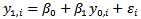 | (1) |
3. Transition Probabilities
- While the presentation of transition probabilities is not new to studies of intergenerational mobility, analysis rarely has extended beyond observation of the raw transition data matrix and has not provided supporting statistical analysis or inference. References[4],[14] and[16], for example, all show discrete transition matrices that indicate little mobility exists at the top of the earnings distribution, but we are unable to determine whether or where the distributions exhibit statistical differences. Statistical evidence remains confined to parameterized results. For example,[14] analyzes a cubic model and rejects of the hypothesis for a linear specification, also indicating that the lowest and highest quartiles have the least mobility for sons. Reference[4] also finds evidence that appear to refute arguments of substantial mobility, finding some upward mobility from the lower parts of the distribution, but top-down mobility appears less substantial.While not analyzing intergenerational mobility,[17] analyzes a transition probability matrix generated through a stochastic kernel and indicates that countries diverge over time into polarized clubs of economic growth. This method of analyzing transition matrices removes arbitrary effects from discretizing the transition matrix and allows for the discovery of emerging twin peaks or convergence clubs in the distribution of cross-country economic growth.Reference[17] use of empirical methods that analyzes distributional anomalies in a continuous framework serves as a starting-point to help understand the evolution of family outcomes across generations. Stochastic kernels visually help indicate the presence of poverty traps and stratification, although the usefulness of this visual inspection may be limited. If stratification exists, members of different social classes will converge to different distributions. We can, however, use the nonparametrically estimated transition matrices to construct stationary distributions and the intergenerational stochastic processes for both whites and African-Americans.The methodology of analyzing stochastic kernels has roots in earlier models of discrete transition matrices. Although not always explicitly stated in studies of intergenerational mobility that analyze transition matrices, each build on the theory of Markov chains in discrete frameworks Examples discussing proofs and basic assumptions comprehensively appear in[18] and[19]. In this discrete framework, pjk is a measure of the probability that the adult-child of a parent from class j is in class k. Since the system is closed, and this is a probability measure, it must be that Σ pjk =1 across all k-classes. If we consider only families in which one son is born to one father, the class history of the family will be a Markov chain. In a real population, this is an implausible assumption where some fathers have more than one son and some fathers have none. If population size remains constant over time, the assumption that on average, each father has one son, or each married couple has two children does not seem implausible. Results from this represent an average set of outcomes for a society with zero population growth.The continuous version of the model outlined in[17] and[20] for understanding distribution dynamics defines the cross-section distribution at time g as Fg, with a probability measure of ϕg. A sequence of probability measures, {ϕg: g ≥ 0}, represents the stochastic process, where the law of motion describes the evolution of the distribution into either a point mass or stratified groups of observations.The dynamics of the stochastic process, {ϕg: g ≥ 0}, satisfy the difference equation:
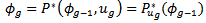 | (2) |
4. Data and Measurement Issues
- A significant barrier to the accurate analysis of economic mobility in earlier studies has been the lack of quality measures for economic outcomes. When regressors contain measurement error in a linear model, attenuation bias distorts estimates of the coefficient of interest. In the context of linear intergenerational mobility, attenuation bias implies an overestimation of economic mobility. In the presence of measurement error in the regressor, researchers do not observe the true value of parents economic outcomes, y0,i. Instead, one observes y0,i* = y0,i + ui. (Measurement error in y1,i appears in the error of (1) and will bias variance estimates, but not the coefficient on intergenerational persistence.) Regressing y1 on y0* through ordinary least squares generates a consistent estimate of β1*=κ β1 where κ, often called the attenuation factor, is less than one. (Most recent graduate econometrics textbooks contain a proof.) This implies that the coefficient for mobility attenuates towards zero (i.e. a linear regression overestimates mobility).The relaxation of the linearity assumption of intergenerational transmissions has led to mixed results in previous research. Responding to criticisms that the models contain intrinsic nonlinearities, many papers including notably[4] and[14] incorporate quadratic or higher-order terms in estimation. By averaging data over several years to reduce attenuation bias, these studies find that higher-order effects often exist, but the results are not conclusive or ubiquitous. Reference[21] also suggests a lack of evidence pertaining to nonlinearities, and completely discounts nonlinear intergenerational models. The discrepancies, however, may be attributable to a simpler result.While[3] and[4] formalize the theoretical effects of measurement error in linear models, the discussion has not received the same attention in nonlinear contexts. To clarify, if a model defines regressors as polynomials, the full effect of using OLS on the coefficients is not simply κ. To see this, consider the quadratic example
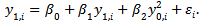 | (3) |
4.1. Average Observed Outcomes
- Since the work of[4] and[5], researchers have dealt with measurement errors in economic outcome variables such as earnings and income through a simple technique of averaging the outcomes over as many years as possible given limitations of data. Average earnings are calculated from Ti years in which we observe data for an individual the ages of 24 and 65. This generates the simple average
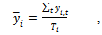 | (4) |
4.2. Average Age-Adjusted Outcomes
- An alternative method for reducing measurement error follows from the empirical model in[23], who estimates life-cycle earnings of fathers using a fixed effect model. Following more closely the theory in the labor economics literature, especially the work of[7] and[24],[23] estimates the age-earnings profiles for various occupations to capture life-cycle parental earnings outcomes, noting that that career choice and timing of human capital investments may affect the general shape of the life-cycle profile. An important contribution of this work is the use of a fixed effect model to capture the heterogeneity across individuals and occupations in age-earnings profiles. Building on[23], I include a simple error specification change which allows for auto-correlated errors in life-cycle outcomes and facilitates correct polynomial specifications. To address problems related to auto-correlation in the estimation of life-cycle earnings, age-outcome profiles for each individual and occupation are estimated using the Baltagi-Wu estimator as outlined in[25]. Not only does this address the different timing of investment decisions across occupations, levels of education and individual specific abilities, but also allows for the auto-correlation in transitory shocks that contribute to measurement error. Occupations include: professionals, managers, clerical/sales, craftsmen, operative, laborer and other. The most general c-order polynomial model, estimated separately for each occupation and generation follows as:
 | , (5) |
 | (6) |
4.3. PSID Data
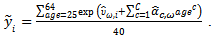
- Data used in the subsequent analyses comes from both the SRC cross-section sample and SEO component of the Michigan Panel Survey of Income Dynamics (PSID) as reported longitudinally from 1967-2003. The PSID includes a vast amount of data collected from family units and individual members of families over the course of a lengthy period of time, beginning in 1968 and continuing until the present. The PSID is particularly useful for analyzing intergenerational mobility on a national scale, since it follows adult children over consecutive years after they leave their parents' households. Ideally it also measures outcomes across generations, which can facilitate the reduction of biases generated from using only a single-year of data. Exploiting this panel structure can generate two alternative measures of earnings. The first method uses the previously discussed simple average of observed annual data, equation (4). The second measure is constructed from age-adjusted predictions as shown above in equation (6). Employment and subsequent data for individuals younger than 25 years and older than 64 is not used. Monetary values are expressed in 1982-1984 dollars measured by the consumer price index for all items. Annual earnings include self-reported money income from wages and salaries earned on all jobs by the individual. For earnings estimates, I exclude individuals with non-positive outcomes. All sons, including those from multi-son households are included in the analysis. Approximately 43% of sons in the sample come from multi-son households Given estimation issues for female earnings associated with fertility choices and sample selection, only the outcomes of sons are analyzed in this paper.To generate age-adjusted profiles, variables are constructed as the natural log of observed earnings for individuals at each point in time. Estimates are generated for 13 separate regressions for fathers' life-cycle earnings based on occupation and education and 7 separate regressions for sons' earnings based only on occupation partitions. Among sons' life-cycle earnings regressions, no statistical difference in parameters exist based on education levels within any of the occupations, but differences exist between occupations. Individuals who indicate more than one occupation over their careers were defined within occupation in which they spent the most years given by the data. Specification tests indicate that polynomial age regressors extend to C=4 for most occupations. Results from life-cycle regressions used to generate (7) are available from the author upon request.
|
 | (7) |
 | (8) |
5. Intergenerational Distributions
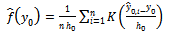
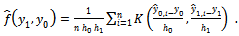
- While simple comparisons of sample means or even regression analysis can reveal information about the conditional mean in the outcomes of a population, the transition probability matrix provides a more generalized description of outcomes. With even more detail, an analysis of distributions generated by a stochastic kernel can reveal whether the children of the rich and poor each face the same distribution of outcomes or fall into poverty traps. The empirical methodology employed for this analysis will estimate the conditional kernels for sons’ earnings
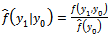 | (9) |
 | (10) |
 | (11) |
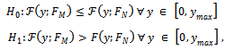
5.1. Testing for Stochastic Dominance
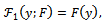
- Analyzing stochastic dominance of the current intergenerational outcomes also can lead to further insight into the structure of nonlinearities. A substantial amount of work on inequality and poverty has tested for stochastic dominance across two independent samples of economic outcomes, usually comparing income distributions at different points across time. None have analyzed outcomes from an intergenerational perspective. Following from[30], tests for stochastic dominance begin with a definition of an operator, Ƒ1(y, F), that integrates F to order k-1. For first orders of operation we have
 | (12) |
 | (13) |
 | (14) |
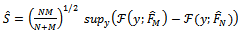 | . (15) |
 . Further details on the construction of S for higher orders of stochastic dominance appear in[30],[31] and[32].
 5.2. Between-Race / Within-Decile Tests
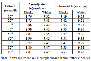
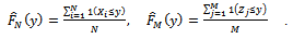
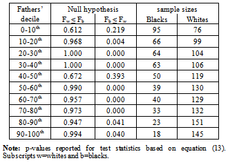
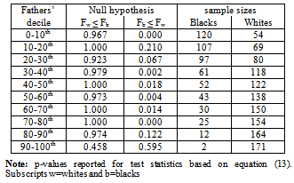
- The unconditional means reported in Table 1 indicate that African-Americans on average have worse outcomes than whites regardless of their fathers' earnings. While these statistically differ, we can ascertain little additional information without a more in-depth analysis. One way to accomplish this is to test for stochastic dominance as outlined in section 5.2. Tests of first-order stochastic dominance within transition matrices generate perhaps the most compelling statistical results with respect to these differences. In particular, differences in between-race earnings not only appear more complex than Table 1 indicates, but evidence supports the conclusion that white distributions stochastically dominate the distributions of African-Americans at nearly all-points between the distributional tails. Tables 2 and 3 report the estimated p-values based on test statistics S (not shown), which we use to conduct inference on the hypothesis given by equation (13). The decision rule rejects the null if p < α. As in parametric inference, large p-values indicate a failure to reject the null. Columns labeled Fb (y) ≤ Fw (y) show p-values for the null hypothesis that African-American distributions weakly dominate white distributions. Columns labeled Fw (y) ≤ Fb (y) give p-values for the null that white distributions weakly dominate African-American distributions. Sample sizes used for tests also appear in the tables. In Table 2 which reports tests based on age-adjusted measures of earnings, results indicate that the distribution of white earnings stochastically dominates African-Americans outcomes for nearly every decile with the exception of the poorest decile, 0-10th and the 40-50th decile. This conclusion is jointly supported by failure to reject the null that white earning distributions dominate African-Americandistributions, and the outright rejection of the null thatAfrican-American distributions dominate white distributions.
|
|
5.3. Within-Race / Between-Decile Tests
- Unless strong within-race mobility exists, or mobility is nonlinear or even exhibits a negative elasticity (as indicated in[5] for poor African-Americans), then within-race distributions should sequentially increase as fathers' earning deciles increase (F10 (y) ≤ F9 (y) ≤ ▪▪▪ ≤ F1 (y)). That is, a lack of mobility implies that the top decile (indexed by 10) should stochastically dominate the ninth decile, which should dominate the eighth decile, and so on. Tables 4-7 report the p-values for these tests. For example, the top half of Table 4 contains p-values for the between decile tests within the African-American data-set of age-adjusted earnings. Continuing the example, the top-left cell reports the p-value (0.567) from the null hypothesis that the 90-100th decile stochastically dominates the 0-10th decile. The bottom half of Table 4 gives the p-value (p=0.161) for the converse hypothesis that the bottom decile stochastically dominates the top decile. To complete the inference, we need and use both results. For statistical evidence that earnings of African-Americans born into the 90-100th decile stochastically dominate the earnings of African-Americans born into the 0-10th decile, the p-value reported in the top half of the table should exceed our cut-off for α. In addition to this, the p-value in the bottom half of the same table should be less than α. Similar reasoning follows for other distributional comparisons. Shaded cells represent one-tailed rejection regions with p-values < 0.05. In summary, less within-race mobility exists when the bottom halves of Tables 4-7 have more shaded cells and the top halves are clear. In contrast, more mobility exists if we observe few statistical differences and where little cell shading exists in the bottom half of a table. Shaded cells in the top halves of Tables 4-7 indicates negative elasticity of intergenerational earnings.
| |||||||||||||||||||||||||||||||||||||||||||||||||||||||||||||||||||||||||||||||||||||||||||||||||||||||||||||||||||||||||||||||||||||||||||||||||||||||||||||||||||||||||||||||||||||||||||||||||||||||||||||||||||||||||||||||||||||||||||||||||||||||||||
| |||||||||||||||||||||||||||||||||||||||||||||||||||||||||||||||||||||||||||||||||||||||||||||||||||||||||||||||||||||||||||||||||||||||||||||||||||||||||||||||||||||||||||||||||||||||||||||||||||||||||||||||||||||||||||||||||||||||||||||||||||||||||||
| |||||||||||||||||||||||||||||||||||||||||||||||||||||||||||||||||||||||||||||||||||||||||||||||||||||||||||||||||||||||||||||||||||||||||||||||||||||||||||||||||||||||||||||||||||||||||||||||||||||||||||||||||||||||||||||||||||||||||||||||||||||||||||
6. Conclusions
- Extending research on intergenerational earnings mobility, the results presented in this paper use nonparametric methods to analyze distributions of sons' earnings. Results indicate that the stationary distribution of whites stochastically dominates the stationary distribution of African-Americans. Additional statistical tests following methods outlined in[30] indicate that the decile-conditioned distributions of white sons' earnings stochastically dominate the distributions of African-Americans from similar economic backgrounds. The distributions of white sons' earnings also improve as fathers' earnings improve. This result does not always exist for African-Americans, who only appear to have distributional dominance from the middle class.Although convergence clubs appear not to exist across the distribution of earnings, African-American and white sons clearly have different outcomes. While not providing a reason for these differences, this descriptive paper adds insight into the complex structure of a seemingly simple but often discussed subject. The two races follow two different stochastic processes in intergenerational earnings.
References
| [1] | F. Galton, “Regression Towards Mediocrity in Hereditary Stature”. Journal of the Anthropological Institute of Great Britain and Ireland, vol. 15, pp. 246-263. 1886. |
| [2] | F. Galton, Hereditary Genius: An Inquiry Into Its Laws and Consequences. Macmillan:London. 1869. |
| [3] | G. Solon, “Intergenerational Income Mobility in the United States”, American Economic Review, vol. 82, pp. 393-408. 1992. |
| [4] | G. Zimmerman, “Regression Towards Mediocrity in Economic Stature”, American Economic Review, vol.82, pp. 409-429. 1992. |
| [5] | S. Cooper S, P. Johnson, S. Durlauf, “On the Evolution of Economic Status Across Generations”. American Statistical Association, Papers and Proceedings”. pp.50-58. 1994. |
| [6] | T. Hertz, “Rags, Riches and Race: The Intergenerational Economic Mobility of Black and White Families in the United States”. In Unequal Chances: Family Background and Economic Success. S.Bowles, H.Gintis, M.Osborne (eds). Russell Sage and Princeton University Press: New York. 2005. |
| [7] | G. Becker, “Human Capital and the Personal Distribution of Income: An Analytical Approach”. Woytinsky Lecture No.1, Institute of Public Administration and Department of Economics, University of Michigan: Ann Arbor, MI. 1967. |
| [8] | G. Becker, N. Tomes, “An Equilibrium Theory of the Distibution of Income and Intergenerational Mobility”. Journal of Political Economy, vol. 87, pp.1153-1189. 1967. |
| [9] | R. Bènabou, “Equity and Efficiency in Human Capital Investment: The Local Connection”. Review of Economic Studies, vol. 62, pp.237-264. 1996a. |
| [10] | R. Bènabou, “Heterogeneity, Stratification, and Growth: Macroeconomic Implications of Community Structure and School Finance”. American Economic Review, vol. 86, pp. 584-609. 1996b. |
| [11] | S. Durlauf, “The Memberships Theory of Inequality: Ideas and Implications”. In Elites, Minorities and Economic Growth, E.Brezia, P.Temin (eds). Elsevier Science B.V.. 1999. |
| [12] | S. Durlauf, “Neighborhood Feedbacks, Endogenous Stratification, and Income Inequality”. In Dynamic Disequilibrium Modelling, W.Barnett, G. Gandolfo, C. Hillinger (eds). Cambridge University Press: Cambridge. 1996. |
| [13] | S. Durlauf, “Spillovers, Stratification and Inequality”. European Economic Review, vol. 38, pp. 836-845. 1994. |
| [14] | H.E. Peters, “Patterns of Intergenerational Mobility in Income and Earnings”. Review of Economics and Statistics, vol. 74, pp.456-466. 1992. |
| [15] | R. Hyson, “Differences in Intergenerational Mobility Across the Earnings Distribution”. Working Paper: UCLA. 1998. |
| [16] | J. Behrman, P.Taubman, “Intergenerational Earnings Mobility in the United States: Some Estimates and a Test of Becker's Intergenerational Endowments Model”. Review of Economics and Statistics, vol. 67, pp.141-151. 1967. |
| [17] | D. Quah, “Empirics for Growth and Distribution: Stratification, Polarization, and Convergence Clubs”. Journal of Economic Growth, vol. 2, pp. 27-59. 1997. |
| [18] | D.J. Bartholomew, Stochastic Models for Social Processes. John Wiley & Sons: London. 1967. |
| [19] | E.Parzen, Stochastic Processes,. Holden Day: San Francisco. 1962. |
| [20] | N. Stokey R.Lucas, R.C.Prescott, Recursive Methods in Economic Dynamics. Harvard University Press: Cambridge, MA. 1989. |
| [21] | C.B. Mulligan, Parental Priorities and Economic Inequality, University of Chicago Press: Chicago. 1997. |
| [22] | J. Kuha, J.Temple, “Covariate Measurement Error in Quadratic Regression”. Unpublished Working Paper. Oxford University. 1999. |
| [23] | A. Minicozzi, “Estimation of Sons Intergenerational Mobility in the Presence of Censoring”. Journal of Applied Econometrics, vol.18, no.3, pp.291-314. 2002. |
| [24] | Y. Ben-Porath, “The Production of Human Capital and the Life-Cycle of Earnings”. The Journal of Political Economy, vol, 75, no. 4.1, pp. 352-365. 1967. |
| [25] | B. Baltagi, P Wu, “Unequally Spaced Panel Regressions with AR(1) Disturbances”. Econometric Theory, vol. 15, pp. 814-823. 1999. |
| [26] | A. Pagan, A. Ullah, Nonparametric Analysis, Cambridge University Press: Cambridge. 1999. |
| [27] | B.U. Park, B.A. Turloch, “Practical Performance of Several Data-Driven Bandwidth Selectors”. Computational Statistics, vol. 7, pp. 251-270. 1992 |
| [28] | S.J. Sheather, M.C. Jones, “A Reliable Data-Based Bandwidth Selection Method for Kernel Density Estimation”. Journal of the Royal Statistical Society, Series B (Methodological), vol. 53, pp. 683-690. 1991. |
| [29] | J. Simonoff, Smoothing Methods in Statistics, Springer-Verlag: New York. 1996. |
| [30] | G.F. Barrett, S.G. Donald, “Consistent Tests for Stochastic Dominance”. Econometrica,vol.71, no.1,pp.71-104. 2003. |
| [31] | D. McFadden, “Testing for Stochastic Dominance”. In Studies in the Economics of Uncertainty, in Honor of Josef Hadar. T.B Fomby, T.K. Seo (eds). Springer:New York, Berlin, London and Tokyo. 1989. |
| [32] | G. Anderson, “Nonparametric Tests of Stochastic Dominance”. Econometrica, vol.64, no.5, pp.1183-1193. 1996. |