1. Introduction

1.1. System Estimation

We have used a system estimation technique to test the effectiveness of the selected macroeconomic policies on important macroeconomic targets to judge their appropriateness. In this section we outline this fundamental simultaneous equations estimation technique in order to rationalise its use.

There are two fundamental methods of estimation for simultaneous equations: least squares and maximum likelihood. There are two approaches within each of these categories: single equation methods and system estimation. The simultaneous equations model used was estimated using three-stage least squares (3SLS) estimation method. It uses the least-squares method and is an instrumental variables method. With it one can estimate some equations without specifying the complete system and do not assume a specific distribution for the errors.

Instrumental variables are predetermined variables used in obtaining predicted values for the current period endogenous variables by the first-stage regression. Instrumental variables estimation methods substitute these first-stage predicted values for endogenous variables when they appear as regressors in model equations. The predicted variables are linear functions of the instrumental variables and the endogenous variable. Normally, the predetermined variablesof the system are used as the instruments. It is possible to use variables other than predetermined variables from ones system of equations as instruments; however, the estimation may not be as efficient. For consistent estimates, the instruments must be uncorrelated with the residual and correlated with endogenous variable.

The technique of 3SLS estimates all of the coefficients of the model, then forms weights and re-estimates the model using the estimated weighting matrix. The first two stages of the 3SLS are the same as in the two-stage least squares (2SLS) but the third stage involves an application of feasible generalized least-squares (FGLS) to the equations in the system [1]. Once the 2SLS parameters have been calculated, the residuals of each equation are used to estimate the cross-equation variances and covariances (the error covariance matrix). In the third and final stage of the estimation process, generalized least-squares parameter estimates are obtained. The 3SLS procedure can be shown to yield more efficient parameter estimates than 2SLS because it takes into account cross-equation error correlations to improve large sample efficiency, as long as cross-equation covariances are not zero. The 3SLS technique is guaranteed by the estimation process that its parameters estimates have smaller variances than their 2SLS counterparts and, according to [2], the gain in efficiency is usually in the neighbourhood of five per cent. Making use of the information concerning the endogenous variables in the system and taking into account error covariances across equations makes 3SLS asymptotically efficient in the absence of specification error.

It is worth mentioning that although system methods are asymptotically most efficient in the absence of specification error, system methods are more sensitive to specification error than single equation methods but, according to [3], in practice models are never perfectly specified in which case it is a matter of judgement whether the misspecification is serious enough to warrant avoidance of system methods. Reference [4] is of the view that 3SLS is an appropriate technique when the right-hand side variables are correlated with the error terms, and there is both heteroskedasticity,¹ and contemporaneous correlation in the residuals.

1.2. Economic Policy Experiences, 1970-1996

This section tells the reader about Uganda’s economic and policy experiences albeit very briefly. A discussion of the main economic developments in Uganda with some summary statistics is outside the scope of the present paper.

Following Uganda’s terrible years of tyranny and economic ruin during Amin’s rule of the 1970s ([5], [6]), the government instituted a programme of recovery during 1981-1984, which was intended to reverse the deteriorating economic conditions. The main objectives of the programme were to restore production and exports, eliminate price distortions, discourage parallel market activities, and curtail expansionary aggregate demand. The programme was based upon huge exchange rate depreciation, more flexible price policies, substantial relaxation of exchange control regulations, greater restraint and discipline on fiscal and domestic credit policies and the rehabilitation of the productive sector.

The political regime of that time ended abruptly, with a military coup in 1985. The civil war intensified in the Lutwa's² subsequent period³ until January, 1986. The declining economic trends which had begun in 1984 continued at an accelerated rate and eroded most of the positive gains which had been achieved during the period 1982-1983.

In 1986 when the National Resistance Movement/Army (NRM/A) government took power, it inherited an economy in ruins ([8], [9]). The policy initially based on direct government controls over the economy [10] was abandoned when a three year Economic Recovery Programme (ERP) was agreed on with the IMF and the World Bank. The main objectives ([11], [12]) and instruments of the ERP were to

1. reduce inflationary impact of the budget deficit by reducing government spending and improved tax administration,

2. improve the balance of payments by increasing producer prices, and

3. increase industrial output by liberalizing trade and directing foreign exchange to imported inputs.

As per the objective of the study, were the above initiatives scientifically grounded and/or were they effective? The rest of the paper is meant to address the above with the help of a system estimation technique.

2. Materials and Methods

2.1. Data

Annual series, 1970 to 1996 were used. Care, for purposes of reliability, was taken to ensure, as far as possible, that data for a particular variable is taken from one source. The large number of variables in the model necessitated the use of different sources of data for different variables, and to this extent there remained an element of inconsistency in the data used. Figures given in local currency were converted into US$ using official exchange rate of the time which also introduced some inconsistency in years when the difference between the official and parallel rates was substantial.

2.2. Model

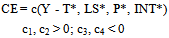
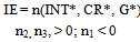
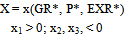
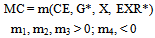
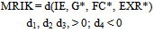
A structural model approach in the tradition of ([13], [14]) was followed where the specific relationships between variables were based (either formally or informally) on economic theory. The usual equilibrium condition of the goods market ensuring that expenditure equals output was the beginning. However, Uganda’s investment and consumption figures did not consistently separate public and private expenditures on these items hence there was likely to be double-counting when government expenditure, investment and consumption were all included. A solution was to exclude government expenditure from the equilibrium condition completely since its expenditure was already included in the aggregated consumption and investment figures.

The Consumption Equation

Disposable income was included as an explanatory variable. Wealth, proxied by money supply, and price were included as arguments in order to capture their effects in line with the permanent income or life-cycle theories of saving and consumption behaviour. The interest rate as a financial determinant of consumption, was included to test its effect vis--vis other variables. Higher interest rates increase the return from saving and also raise the cost of borrowing for large expenditures, thereby reducing consumption. A higher interest rate, other things being equal, was expected to be associated with more savings and less consumption.

The Investment Equation

Investment is the sum of private investment and government investment. Following the neoclassical theory of investment behaviour, the desired level of private capital stock is determined from conditions of profit maximization⁴ subject to a production function. The interest rate entered the investment function also to test its effect. Although neo-classical theory would dictate the inclusion of the price of investment goods, this was not done due to data difficulties.

In Uganda, the desired and the actual capital stock, among other things, depends on retained earnings and credit. One of these two variables, retained earnings, was not included in the investment function because of data difficulties but credit was.

It was assumed that government investment expenditure was positively related to total government development expenditure. The contribution of public fixed investment to total domestic fixed investment was captured by this variable. However, in cases where there are revenue constraints and/or fixed expenditure, government expenditure may be an inappropriate proxy for its investment. Nonetheless, government development expenditure, proxied by government expenditure, as a variable was included.

The Export Function

Exports were assumed to be a function of growth of output of the major importing countries, proxied by OECD average growth rates, with a positive coefficient. The importance of the exchange rate is well specified in the literature and price was specifically included in its own right.

The Imports of Consumer Goods Function

The desired level of imports of consumer goods was hypothesized to be functionally related to the volume of consumption expenditure (private and public⁵), government recurrent expenditure, proxied by government expenditure,⁶ exports as a measure of import capacity, and the exchange rate. The exchange rate was likely to capture some of the effects of the prices for imports of consumer goods as a separate variable.

Import control policies may be proxied by export revenue of the previous period plus net of debt repayment obligations external debt commitments. An increase (decrease) in net foreign exchange position in the previous period is expected to lead to a liberalisation (tightening) of import controls. This lagged contribution or measure of import capacity was not included in the specification but some elements of its effect were captured by exports as a measure of import capacity.

Parallel market exchange rate premia can be used as an index of regulation [18]. Exchange rate premia⁷ correlate well with the past history of regulation and, therefore, serve as a reasonable proxy of the regulatory environment. This, however, was not a fully satisfactory measure of regulations because it may simply be capturing the effects of import restrictions. Since it could be import restrictions that we are primarily interested in here, this can be a useful proxy but not included in the specification.⁸

The Import Demand Function for Investment Goods

In this specification, the desired level of imports was hypothesized to be functionally related to total investment expenditures in the economy, foreign capital inflow, and the exchange rate. Including its development expenditure, proxied by government expenditure, captured the involvement of government in importing capital goods. Including foreign capital inflow as a variable captured the importance of foreign capital. The justification for the inclusion of the exchange rate as an explanatory variable in an import demand function was spelt out earlier.

Since few capital goods are produced domestically and, moreover, since most imported investment goods are non-competing with domestic investment goods, the price of domestic investment goods was not introduced as an argument. The speed of adjustment coefficient was hypothesized to be functionally related to the foreign exchange position of the previous period but not included as an argument because some of the relevant effects were captured by foreign capital inflows given the circumstances in Uganda. Lagged investment goods or inputs imports could be added as an argument or arguments ([20], [21]) but was/were not.⁹

Specification

We now specify the overall structure of the model, including the functional form for each equation. It consists of five (5) stochastic or behavioural equations, six (6) endogenous variables and nine (9) exogenous variables that help to cause the movement of the endogenous variables in the system.¹⁰A variable with an asterisk is an exogenous variable, while a variable without an asterisk is an endogenous variable. The basic information in this model is summarized below:

(1)

(2)

(3)

(4)

(5)

(6)

The endogenous variables

CE = Consumption expenditure per capita in current US$.

IE = Fixed investment/capital formation per capita in current US$.

MC = Imports of consumer goods per capita in current US$.

MRIK=Imports of raw materials, intermediate goods, and capital goods per capita in current US$.

X = Total exports per capita in current US$.

Y = Income per capita in current US$.

The exogenous variables

CR* = Bank credit to the private sector per capita in current US$.

EXR* = Exchange rate, i.e. units of domestic currency per unit of foreign currency (Ug Shs/US$).

FC* = Foreign capital inflow per capita in current US$.

G* = Government expenditure per capita in current US$.

GR* = OECD countries’ average growth rates.

INT* = Real nominal (regulated¹¹) less inflation rate of interest.

LS* = Money supply per capita in current US$.

P*= Retail price level or retail consumer index.

T*= Tax per capita in current US$.

In order to calculate 3SLS estimates, our specification had to and indeed did satisfy the order condition for identification which, according to [26], says that “there must be at least as many instruments, including the constant, in each equation as there are coefficients (right-hand side variables) in that equation”. Reference [27] puts it that “the order condition states that if an equation is to be identified, the number of predetermined variables excluded from the equation must be greater than or equal to the number of included endogenous variables minus one.” They further state that “a necessary condition for an equation to be identified is that the number of all variables excluded from the equation be greater than or equal to the number of endogenous variables in the model system.”

2.3. Testing and Evaluation

For purposes of model testing and evaluation, tests of significance of the estimated coefficients were used to validate the model or to bestow some degree of credibility to it. In addition, conclusions were drawn on the basis of the degree of explanatory power of each equation (R² and adjusted R²), direction and size of impact of an independent variable (respective coefficient sign and size) as well as its statistical significance, and significance of each equation’s independent variables on the dependent variable (F value). Evaluation was also based on the statistical “fit” of individual equations to the data (root MSE).

F-values test the significance of the self-determining variables on the dependent variable, that is, “the F test on R² provides a test of the null hypothesis that all regression coefficients are zero” [28]. The F-test shown in the instrumental variables case is a valid test of the no-regression hypothesis that the true coefficients of all regressors are zero, that is, all the non-intercept parameters. However, because of the first-stage projection of the regression mean square, this is a Wald-type test statistic, which is asymptotically F but not exactly F-distributed in finite samples. Thus, for small samples the F-test is only approximate when instrumental variables are used.

The coefficient of determination, R², (in some cases adjusted for the degrees of freedom) compares the errors of the regression predictions with those of the mean predictions [29]. It is generally viewed as the proportion of variation of the dependent variable that is explained by the regression. The higher the proportion, the greater is the explanatory power. It has a tendency of being higher for time series than for cross section analysis because of the existence, by definition, of time-trend in the data which pushes it up.

The R² statistics when the results are based on predicted values for the endogenous regressors from the first-stage instrumental regressions is difficult to interpret [30]. When instrumental variables are used, the regression sum of squares (RSS) and the error sum of squares do not sum to the total corrected sum of squares. In this case, there are several ways the R² statistic can be defined. The definition of R² used by the SYSLIN procedure utilized in this study is

.

This definition is consistent with the F-test of the null hypothesis that the true coefficients of all regressors are zero. However, this R², according to [31], may not be a good measure of the goodness of fit of the model. In other words, R² is valid for hypothesis tests but may not be a good measure of fit for models estimated by instrumental variable methods.

Root mean square error for the model (Root MSE) is an estimate of the standard deviation of the error term. The RMS error¹² is evaluated by comparing it with the average size of the variable in question. It facilitates comparison between the actual and predicted endogenous values - if the predicted series is a good approximation to the actual series, we expect it to be small (zero in case of perfect fit).

In a system method like the 3SLS used, the system weighted MSE and R² measure the fit of the joint model obtained by stacking all the models together and performing a single regression with the stacked observations weighted by the inverse of the model error variances. In case of this study, they were 0.9675 with 112 degrees of freedom and 0.9968 respectively.

Table 1. Likelihood Ratio Versus Theoretical Values Series: CE YD LS P INTLags interval: 1 to 2 Series: IE INT CR GLags interval: 1 to 3 Likelihood Critical Values Likelihood Critical Values Ratio 5 Percent 1 Percent Ratio 5 Percent 1 Percent 138.3292 68.52 76.07 109.7054 47.21 54.46 73.63876 47.21 54.46 35.86105 29.68 35.65 30.64697 29.68 35.65 14.86853 15.41 20.04 10.24946 15.41 20.04 5.539670 3.76 6.65 0.765411 3.76 6.65 Series: X P EXR GRLags interval: 1 to 2 Series: MC CE G X EXRLags interval: 1 to 2 Likelihood Critical Values Likelihood Critical Values Ratio 5 Percent 1 Percent Ratio 5 Percent 1 Percent 199.1932 47.21 54.46 155.4501 68.52 76.07 33.12677 29.68 35.65 77.28902 47.21 54.46 12.68422 15.41 20.04 24.14792 29.68 35.65 1.078590 3.76 6.65 6.266612 15.41 20.04 0.466813 3.76 6.65 Series: MRIK IE G FC EXRLags interval: 1 to 2 Likelihood Critical Values Ratio 5 Percent 1 Percent 136.9842 68.52 76.07 73.14996 47.21 54.46 34.83193 29.68 35.65 11.69285 15.41 20.04 0.204695 3.76 6.65

First-order serial correlation¹³ is the problem in which errors in one time period are correlated with errors in the ensuing time period. Durbin-Watson (D-W) test is one of the most popular in testing for first-order autocorrelation and, according to [32] “by far the most popular test for serial correlation.”

Accepting or rejecting a particular result may call for additional analysis based upon a Durbin-Watson statistic reported as indicative of the presence or absence of serial correlation in the residuals of an estimated equation. It can be corrected, for instance, by modifying the original specification to take account of the serial correlation. This can be done if we include lags of the independent variables or include autoregressive (AR) and/or moving average (MA) terms in the equation. If not corrected, serial correlation in the residuals will lead to incorrect estimates of the standard errors, and invalid statistical inference for the coefficients of the equation. Though, according to [33], a Durbin-Watson statistic can be difficult to interpret, one thing is sure: when it is too low (close to zero) it suggests that the variables are not co-integrated and the results spurious.

It is now common practice to undertake time series analysis by looking at time series characteristics of the data. This includes tests for stationality and co-integration. Through Durbin-Watson test and likelihood ratio versus theoretical values (Table 1), the variables are co-integrated. Further, the structural relationships described by the equations are invariant over time, that is, stationary.

3. Results

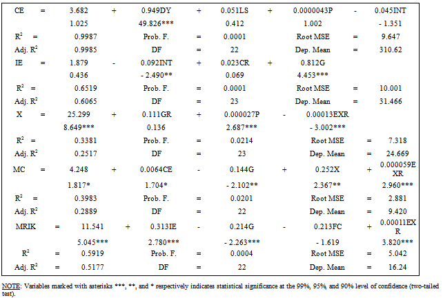
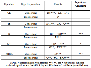
Estimation of the model using 3SLS method results are summarized in tables 2 and 3. The estimation results can be considered to be fairly good because, in general, the parameters in the model have signs that conform to our expectations with a number of coefficients that are statistically significant.

In the consumption expenditure equation, disposable income was statistically significant at 99 per cent level of confidence with the expected sign. For the investment expenditure (fixed investment/capital formation) equation, two of the three variables were statistically significant at the reported levels, and all variables had the expected signs. Government expenditure was statistically significant at 99 per cent level of confidence and the real lending interest rates at 95 per cent. With regard to the export equation, it is only GR that was not statistically significant at the reported levels of confidence though with an expected sign. The EXR was statistically significant at 99 per cent level. The general price level was statistically significant at 99 per cent level but with an unexpected sign. Though the fit of the import of consumer goods equation was relatively poor, all variables in the equation were statistically significant at the reported levels of confidence but half of them with unexpected signs, namely the government expenditure and the exchange rate which, other things being equal, we should be concerned about. For the imports of raw materials, intermediate and capital goods equation, it is only the foreign capital that was not statistically significant at the reported levels of confidence. Besides the constant, investment expenditure remained the most relevant variable at 99 per cent level of confidence, and with a positive expected sign. Like in the case of the import of consumer goods, both government expenditure and exchange rates were statistically significant at the reported levels but had unexpected signs.

Table 2. SAS 3SLS Estimation Results

Table 3. SAS 3SLS Basic Significance Tests and Sign Expectations

4. Discussion and Conclusions

We now turn to a brief discussion of the results and their implications. The macroeconomic model focused on joint determination of consumption expenditure (CE), investment expenditure (IE), exports (X) and imports, that is, imports of consumer goods (MC), and imports of raw materials, intermediate and capital goods (MRIK). The basis for their joint determination was partly already established. In line with the objectives of the study, the discussion focuses on the macroeconomic model results’ relevancy to Uganda’s policy experiences of Amin (1971-1979), Obote II (1980-1985), and Museveni I (1986-1995) regimes in Uganda using the data set period 1970-1996.

We can examine the dynamic characteristics of our macroeconomic model by looking at the impact effects of changes in the exogenous variables on the endogenous variables - the coefficients. This helps us to comment on the behaviour of the Uganda economy and the effects of the policies on consumption, investment, exports and imports in Uganda. We can, for instance, conclude, on the basis of the macroeconomic model investment equation (Table 2) that the impact effect of a dollar increase in government expenditure per capita was an increase in investment expenditure by about US$0.80 per capita.

In general our findings suggests that for consumption expenditure (CE), disposable income (DY) was the most relevant policy variable and that while the general price level (P) was not so relevant, it had a positive effect. This lends credence to the ERP policy of reducing government spending.

Since the level of investment is endogenous, our macroeconomic model can explain medium-term growth and it was shown that it is heavily positively dependent on two policy instruments namely government expenditure (G) and the real lending rate of interest (INT). It is shown that in Uganda a rise in the interest rates displayed the orthodox (contractionary) effects rather than the McKinnon-Shaw (expansionary) effects.¹⁴

The exchange rate (EXR) policy instrument, in general, dominated the external sector and affected the export sector in an expected fashion. The general price level in Uganda at the time was also relevant to the export sector though it did not seem to reduce exports when it increased, supporting the then ERP policy of increasing producer prices.

For the import sector, on the other hand, the influence of the exchange rate was different – it was positively related to imports. This means that its increase could not reduce imports of any kind! In addition to the exchange rate, government expenditure (G) is shown to have been an effective policy variable for all types of imports but in an unanticipated manner. Increased government expenditure seems to have led to a reduction in imports contrary to what one would expect.

Overall the ERP policies of the time were, in some respects, empirically validated with respect to consumption expenditure and exports while the behaviour of the economy in general also conformed to expectations in the literature like the contractionary effects of the interest rate.

Notes

1. As opposed to homoscedasticity which assumes that the error term has constant variation, heterskedasticity though less common assumes changing error variation for different equations.

2. Lutwa (RIP) was the president who took over from Obote II.

3. Okello-Lutwa fiasco is found in [7].

4. This need not be the case for all government fixed capital some of which may be influenced by some social welfare function. This was not directly included except in as far as it was captured by government development expenditure, proxied by government expenditure.

5. Bledjer and Cheasty [15] emphasize that "the government, even if infinitely lived, is constrained - like private consumers - by the size of its permanent income." They note that both its wealth and its income determine a government’s consumption.

6. Tanzi [16] expresses the view that "the dividing line between what is classified as recurrent and what is classified as capital expenditure is, in the real world, an arbitrary one that can be moved up and down depending on the picture that the policy-makers may wish to present to the world”. In broadly a similar tone, [17] argues that the components of government spending are policy-determined.

7. Exchange rate premia is defined by [19] as

where

8. Import restrictions ceased to be a big issue in Uganda when a Bank/Fund programme started in 1987. Also it was a non-issue during the Bank/Fund programme 1981-1984.

9. Reference [22] used the lagged dependent variable coefficient as a partial adjustment coefficient and interpreted another’s size and significance as a reflection of considerable inertia.

10. This is relatively a small model – ”larger models may be more realistic and preferable as descriptions of reality” [23]. To some extent this was dictated by paucity of data on the Uganda economy. Also it may not be a sensible way to construct a huge model to handle all aspects of macroeconomic effects in one short. Each model type has its own advantages and disadvantages, and the advantages can best be attained in a simpler and clearer form. Reference [24] argues that “sometimes reducing the size of a model improves its forecast performance and that the amount of detail involved in a model depends on the intended uses” [25].

11. Market after its liberalisation in late 1992.

12. Mean square error combines bias and variance.

13. There are many orders of serial correlation, one or first being the most popular or commonly tested.

14. In light of [34] and [35], and the critique in [36].