-
Paper Information
- Next Paper
- Paper Submission
-
Journal Information
- About This Journal
- Editorial Board
- Current Issue
- Archive
- Author Guidelines
- Contact Us
American Journal of Economics
p-ISSN: 2166-4951 e-ISSN: 2166-496X
2012; 2(5): 61-74
doi: 10.5923/j.economics.20120205.01
The Landscape of Poverty in Nigeria: A Spatial Analysis Using Senatorial Districts- level Data
 Abstract
 Reference
 Full-Text PDF
 Full-Text HTML
Sowunmi F. A. 1, Akinyosoye V. O. 2, Okoruwa V.O. 2, Omonona B. T. 2
1Department of Economics, Lagos State University, Lagos, Nigeria
2Department of Agricultural Economics, University of Ibadan Ibadan, Nigeria
Correspondence to: Sowunmi F. A. , Department of Economics, Lagos State University, Lagos, Nigeria.
| Email: |  |
Copyright © 2012 Scientific & Academic Publishing. All Rights Reserved.
The study decomposes the Landscape of Poverty in Nigeria based on the significance of spatial contiguity using Senatorial Districts - level Data. The data used for the study were obtained from National Living Standard Survey and Core Welfare Indicators Questionnaire Survey conducted by National Bureau of Statistics in 2004 and 2006 respectively. Exploratory spatial data analysis and spatial autocorrelation test were carried out on poverty incidence data. Average national poverty rate of the Senatorial Districts (SD) was 56.0%. Forty nine percent of the SD had poverty rate (PR) below the national average. The global Moran’s I value obtained is strongly positive (0.6657), indicating that spillover of poverty exist among SD. The study revealed that 52% of the SD with significant spatial association had low PR neighboured by low PR SD (Low-Low), 41% of the SD with high PR were neighboured by high PR SD (High-High) and 7% of SDs with low PR were surrounded by high PR SD (Low-High). The mean PR in high-high and low-low SDs was 82.6% and 31.8% respectively. The study recommends that for a significant poverty reduction to be achieved in Nigeria, greater attention in terms of poverty alleviation strategies should be concentrated on the senatorial districts that constitute the hotspots of poverty.
Keywords: Spatial Contiguity, Poverty Rate, Spatial Autocorrelation, Senatorial District
Article Outline
1. Introduction
- The poverty phenomenon in Nigeria and other developing nations has attracted significant global attention since the 1990s. First, was the annual publication of the Human Development Report by the United Nations Development Programme (UNDP) which contains estimates of the Human Development Indices used to rank all the 177 Countries that make up the United Nations. The Human Development Index (HDI) is derived from social and economic indicators that are closely correlated with poverty. Human Development Index is a simple summary measure of three dimensions of human development concept: living a long and healthy life, being educated and having a decent standard of living. Thus it combines measures of life expectancy, school enrolment, literacy and income[1]. Since 2003, African Countries including Nigeria have ranked amongst the countries with the lowest HDI. In 2005, all the 27 Countries of the world with the lowest HDI were African Countries, Nigeria inclusive. These countries each has HDIs of less than 0.5 and when compared with figures of 0.968 for Iceland and Norway (the countries with the highest HDI) one will realized the enormity of the poverty problem in Nigeria and other lowly developed African Countries. Though the issues of poverty and low human development indices may not be peculiar to Africa, they are however more pronounced in the continent and the Nigeria situation is particularly worrisome because of the country’s available natural resources and clement weather. Despite the conflicting statistical data on the incidence of poverty between government agency and international organization, there is undeniable fact that poverty situation in Nigeria is serious and deserves great attention. Specifically,[2] put the poverty rate of Nigeria at 54.4% while[1] and[3] reported 70.2% and 70% respectively. Over the years a number of Poverty Reduction Strategy Programmes (PRSPs) has been initiated in Nigeria, this includes the recently designed National Economic Empowerment Development Strategies (NEEDS. In addition to the foregoing, a special Federal Government institution to alleviate poverty in the country; the National Poverty Eradication Programmes (NAPEP) was created. These previously initiated PRSPs in the country along with many others initiated by the state governments appear only to have addressed the various manifestations of poverty, such as unemployment, lack of access to credit and functional rural and urban infrastructures, and gender inequality among others. While the above mentioned Poverty Reduction Strategy Programmes (PRSPs) were well intentioned, none had any significant, lasting, or sustainable positive effects on the people they were planned for[3],[4]. This can be attributed among others to the non consideration of the heterogeneous nature of poverty and spatial contiguity of geographical units in the design of PRSPs. Existing poverty studies treat a geographical unit, such as a local government area, a state, or a senatorial district, or a county, as an independent isolated entity rather than as an entity surrounded by other geographic units with which it may interact is being considered by this study. Moreover, there is scarce information on spatial decomposition of poverty incidence among SD in Nigeria. Hence, the landscape of Poverty in Nigeria is investigated using Senatorial Districts (SDs) in Nigeria as geographic units. Senatorial district is composed of Federal constituencies while federal constituency is made up of Local Government Areas. Each state is made up of three senatorial districts while the federal capital territory (Abuja) has one senatorial district. This means that each state in Nigeria is represented by three elected senators in the national assembly (upper legislative chamber). Delineation of the country into senatorial district by National Population Commission is based on population distribution. Apart from performing the legislative duties, senators are also task with the economic development of their respective senatorial district through lobby for sitting capital projects and judicious use of monthly constituency allowance meant for execution of projects in senatorial districts. The study utilized spatial econometrics technique instead of the conventional econometrics methods. Spatial econometrics technique has the advantage of addressing the problem of spillover effect or spatial autocorrelation if present in the data set. According to[5], studies that ignore spatial autocorrelation (dependence) can produce biased results (coefficient estimates) and lead to ineffective and possibly counterproductive – recommendations for policies targeted at poverty alleviation. The study identified the locations of senatorial districts with similar and dissimilar (outlier) pattern of poverty incidence. Knowing this will afford researchers to determine the factors that are specific to each of the identified groups. The finding of this study is expected to assist government in localizing poverty alleviation strategy of senatorial districts that exhibit similar spatial pattern of poverty.
2. Conceptual Framework and Previous Literature
2.1. Conceptual Framework
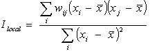
- The philosophy behind this study is based on Tobler First Law of Geography:"everything is related to everything else, but near things are more related than distant things." Spatial clustering shows the similarity or dissimilarity of poverty in neighbouring units and spatial autocorrelation measures the strength of the spatial clustering[6],[7],[8],[9],[10]. Global spatial autocorrelation (Moran’s I) analysis yields only one statistics to summarize the pattern of poverty in the whole study area. That is, global Moran’s I assumes homogeneity of the study area (that poverty pattern is the same in all the senatorial districts). This is the limitation of global Moran’s I. To localize the presence and magnitude of spatial autocorrelation, a measure such as Anselin’s Local Indicators of Spatial Association (LISA) is necessary (see equation 7). This approach is most useful when, in addition to global trends in the entire sample of observations, there exist also pockets of localities exhibiting heterogeneous values that do not follow the global trend. This leads to identification of so-called hot spots -regions where the considered phenomenon is extremely pronounced across localities- as well of spatial outliers[11]. ‘Moran scatter plot’ plots a variable of interest against spatial weighted component of that variable. This measure permits a more disaggregated view of the type of spatial autocorrelation that exists in a data. Local Indicators of Spatial Association[12] and Moran scatter plot[13] are valuable for gaining a ‘‘local’’ understanding of the extent and nature of spatial clustering in a geographical unit. LISA indicates significant spatial clustering for each location.Moran scatter plot utilizes graph only to identify observations (extent of poverty) that are similar as well as different (outliers: neighbouring senatorial districts that has contrasting poverty rates) from their neighbours while formula is used in Local Moran’s I to identify similarity or dissimilarity of poverty rates in neighbouring units. For each location (senatorial district), LISA values allow for the computation of its similarity with its neighbours and also to test its significance. Spatial association can be decomposed into four components, viz: ■ Senatorial districts with high concentration of poverty with similar neighbours: high-high. Also known as “hot spots”.■ Senatorial districts with low concentration of poverty with similar neighbours: low-low. Also known as “cold spots”.■ Senatorial districts with high concentration of poverty with low concentration of poverty neighbours: high-low. Potential “spatial outliers”.■ Senatorial districts with low concentration of poverty with high concentration of poverty neighbours: low-high. Potential “spatial outliers”.■ Senatorial districts with no significant local autocorrelation.Reference[13] demonstrated that the slope of the regression line through the points in Moran scatter plot expresses the global Moran’s I value. A strong positive statistic indicates positive spatial autocorrelation (clustering of like values). This means that most senatorial districts would be found in the high-high or low-low (first and third quadrants) areas of the country. A strong negative statistic indicates negative spatial autocorrelation suggests most senatorial districts with high (low) poverty concentration would be found in the vicinity of low (high) poverty senatorial districts (outliers).
2.2. Review of Previous Literature
- Poverty is not only a state of existence but also a process with many dimensions and complexities. Generally, poverty has attracted a lot of attention from the academia and non-academia globally. Few recent studies are based on the premise that individuals and households with common characteristics sometimes are found clustered together either by choice or because they are constrained to co-locate by coercive operation of social, economic, geographic or political forces[14]. Identification of these households has been made possible through the advancement in spatial analytical techniques; which has also enables spatial pattern of poverty (concentration of poverty rates and outliers) to be quantified[15],[16],[17]. References[18],[19] showed that poverty rate in nearby locations are likely to be similar to one another, or error for the model in one area or location is correlated with the error terms in its neighboring locations; hence the need to pay attention to the structure of spatial dependence or autocorrelation in our data. Reference[20] posited that knowing precisely where concentration of poverty exit will help the policy maker, social scientist and all other stake holders in continuing challenge of combating this fundamental threat (poverty) to well-being. Ignoring spatial autocorrelation will make it: ■ impossible to measure the strength of spatial concentration of poverty. ■ difficult to explain substantial variation in the incidence of poverty across senatorial districts.In a study on the topography of poverty in US,[20] findings showed that 51.9% of the total counties belong to similar spatial concentration (low – low and high-high), whereas only 7.8% were categorized as being spatial outliers (high – low and low – high). The remaining 40.3% were neither. The categorization of spatial concentration into high or low poverty rate neighbourhood is in relationship with average national poverty rate. Most counties in US are found in the high-high and low-low subregions[14]. That is, the counties whose poverty rate is above (below) the average poverty rate are surrounded by counties with poverty rate above (below) average national poverty rate. Reference[21] conducted a research on the application of a spatial regression model to analysis and poverty mapping in Ecuador; their results confirmed the significant effects of spatial autocorrelation variable that denotes the presence of clusters in the spatial distribution of poverty and the influence between neighbourhood households on the probability of being poor. A combination of processes (socioeconomic, political, demographic and geographic) operating in space over time has somehow conspired to partition countries into large regions of high and large regions of low poverty—with occasional ‘‘island’’ geographic units here and there that are very different from their neighbors[14].Similarly,[22] in study on spatial clustering of rural poverty in Sri Lanka found that Divisional Secretariat (DS) divisions with a high percentage of poor households are found in four rural districts where agriculture is the main source of livelihood of the majority of households. The clustering of DS divisions of low poverty around major urban centres suggests that, in predominantly agricultural areas, poor people have only limited economic opportunities to escape poverty. They revealed that availability of and access to water and land resources are the major factors of spatial concentration of poverty in rural areas. In another study on spatial approach to social and political forces as a determinant of poverty in US,[5] stated that a positive and significant spatial dependence in the dependent variable (poverty rate) indicates that the poverty rate in a particular county is associated with poverty rates in surrounding counties/local government areas. According to them, the value of the spatial autocorrelation coefficient (ρ = 0.21 in the model for all counties) obtained indicates that a 10 percentage point increase in the poverty rate in a county results in a 2% increase in the poverty rate in a neighbouring county. This is strong evidence that spillover effects exist between counties with respect to poverty. This finding is corroborated by[23]. They reasoned that poverty of a neighbourhood is tied to the fortunes of neighbouring areas: there are geographic spillovers in poverty reduction. Reducing poverty in particular neighbourhoods affects the poverty of neighbouring tracts.
3. Methodology
3.1. Study Area
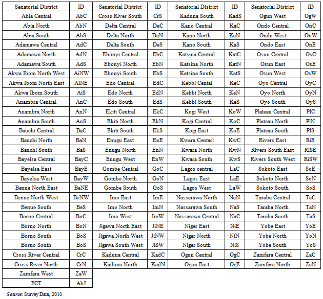
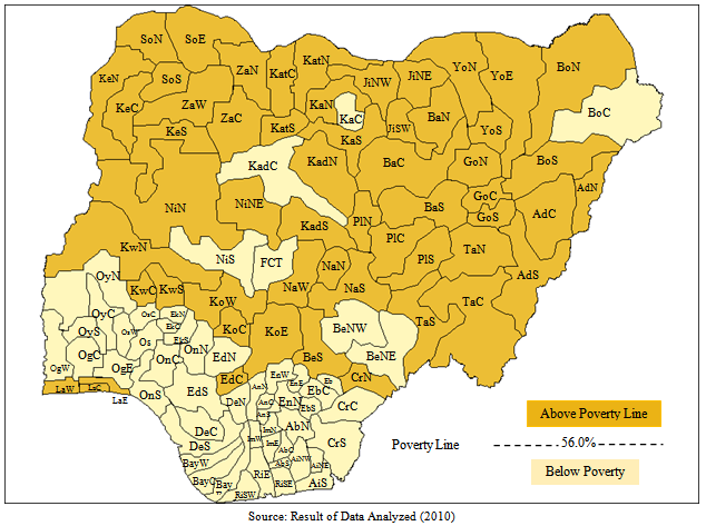
- The study covered the 109 Senatorial districts of Nigeria. According to section five subsections 71 and 72 of Nigeria’s 1999 constitution, “the Independent National Electoral Commission shall divide each state of the federation into three Senatorial districts………. No Senatorial district or Federal constituency shall fall within more than one state, and the boundaries of each district or constituency shall be as contiguous as possible and be such that the number of inhabitants thereof is nearly equal to the population quota as is reasonably practicable.” The fig. 1.0 shows the senatorial district map of Nigeria while table 1.0 gives the meaning of the senatorial districts’ acronyms.
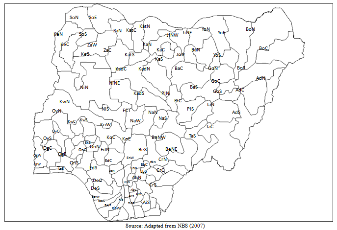 | Figure 1. Senatorial District Map of Nigeria |
3.2. Methods of Data Analysis
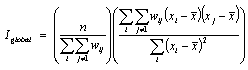
- The study utilized descriptive and exploratory spatial data analyses (ESDA). The GIS software (ArcGIS 8.1) was used to ensure the compatibility of the senatorial district map with Geoda 0.9.5i The most common measure of spatial autocorrelation, a statistic called global Moran’s I[24],[25] is defined as follows:
 | (1) |
 | (2) |
 | (3) |
 | (4) |
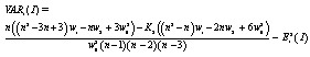 | (5) |
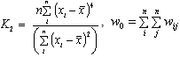 ,
,
|
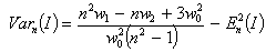
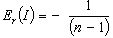
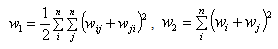 wi. and w.i are the sum of the row i and column i of the weight matrix respectively.The test of the null hypothesis that there is no spatial autocorrelation between observed values over the n locations can be conducted on the basis of the standardized statistics as follows:
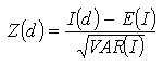 | (6) |
 | (7) |
4. Empirical Results and Discussion
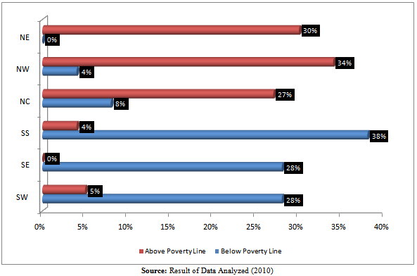
- The study showed a low poverty incidence (%) in the southern part of the country which ranges from 8.1 to 36.9. In the north central, the poverty incidence ranges from 55.4% to 78.1%. The core north which (comprises of north west and north east) has the highest poverty incidence ranging from 78.4 % in Zamfara central to 97.7% in Jigawa northeast. Generally, the study revealed an average poverty rate of 56.04% among the 109 senatorial districts (see figure 1.1). Federal Capital Territory, Kaduna central, Kano central and Borno central are the three senatorial districts in the north that the poverty rates are substantially lower than the national poverty rate. This may be attributed to the location of state capitals (seat of government) in these senatorial districts where basic infrastructures are concentrated. Moreover, the three senatorial districts in Lagos state (Lagos east, Lagos west and Lagos central), one in Edo state (Edo central) and Cross – River (Cross – River north) have the poverty rates higher than the national poverty rate in the south. The poverty rates in the six geopolitical zones corroborate the findings above (see figure 1.2). Specifically, the average poverty rate in the southeast is the lowest (29.9%), while average poverty rates of southsouth and southwest are 39.8% and 37.9% respectively. The northwest geopolitical zone has the highest average poverty rate (77.6%); this is followed by northeast (74.5%) and northcentral (68.1%). The high average poverty rates in the northern geopolitical zones may be attributed to long – standing lags in provision of health, education and other social services resulting in proportionately more poor in the north[28]. He reasoned that the southern zone has most of the industries and many export crops while the northern zone is largely rural and agricultural with a fragile agro – climatic environment and a different socioeconomic history.
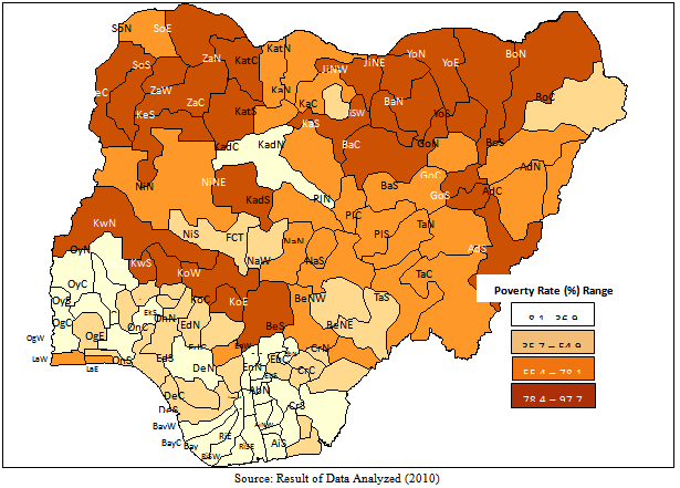 | Figure 1.1. Map of Poverty Rates based on 109 Senatorial Districts |
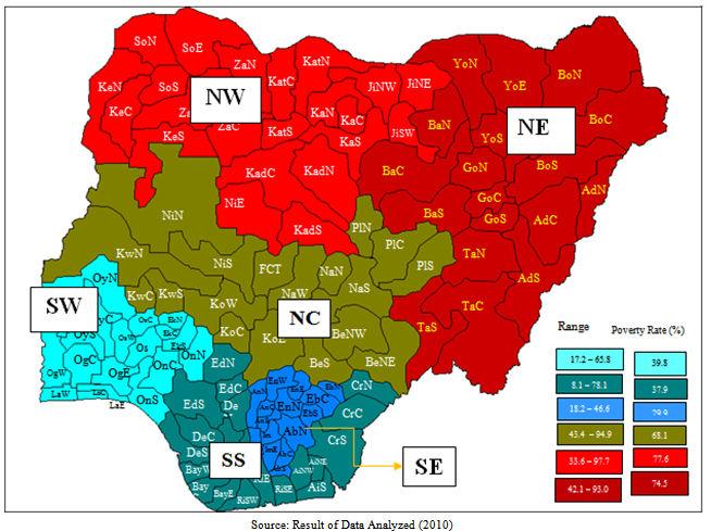 | Figure 1.2. Map of Poverty Rates among the Geopolitical Zones |
 | Figure 1.3. Map of Poverty Line among 109 Senatorial Districts |
 | Figure 1.4. Distribution Poverty Line among Senatorial Districts |
|
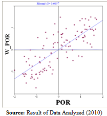 | Figure 1.5. Moran Scatter Plot of Poverty Incidence |
4.1. Location of Senatorial Districts with Similar Pattern of Poverty Incidence.
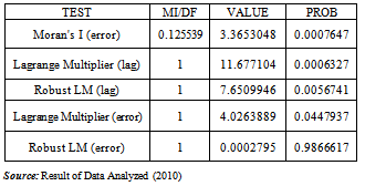
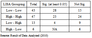
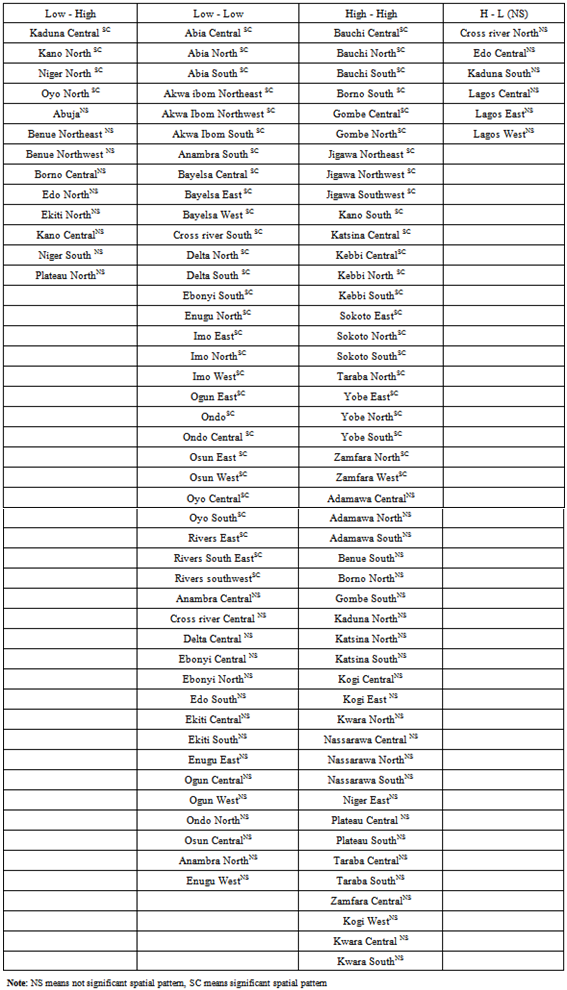
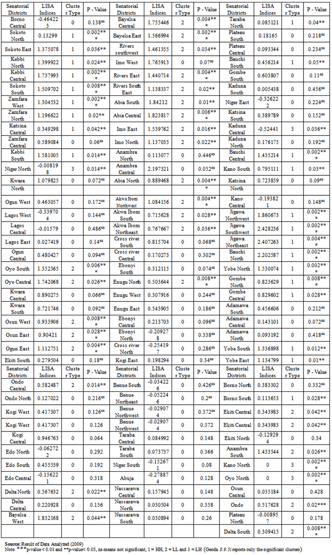
- The result obtained from Local Indicator of Spatial Association (LISA) revealed that out of 90 senatorial districts that have similar spatial pattern of poverty incidence (high-high and low-low), 51 have similar spatial patterns that are statistically significant (at p≤ 5%, see table 1.2 below). The high – high constitutes the senatorial districts with more pronounced poverty incidence as well as their neighbouring SD.
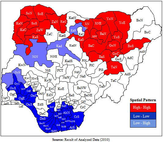 | Figure 1.6. Local Indicator of Spatial Association (LISA) Map for Significant Spatial Pattern |
|
|
|
5. Conclusions and Recommendations
- The application of spatial data analysis methods revealed strong evidence of spatial interaction across senatorial district boundaries. Using a binary weight matrix in the estimation of spatial effects, we found that proximity to senatorial districts that have a high (low) poverty rate will increase the probability that household in a senatorial district will itself have a high (low) incidence of poverty.The landscape of poverty incidence obtained from the study identified the hot spots and cold spots of poverty in Nigeria. Knowing precisely where concentrations and isolated islands of poverty exist will help various government owned organizations with the mandate of alleviating poverty (NAPEP, NEPAD and NEEDS) and state governments in their continuing challenge of combating this fundamental threat to well-being and economic development of Nigeria. Moreover, this finding will assist government agencies saddled with poverty alleviation in applying specific strategy to different landscape of poverty. Also, the elected representatives (senators) are afforded the opportunity of knowing the poverty landscape of their respective senatorial districts so that their constituency development fund can be property channeled to poverty alleviation.
ACKNOWLEDGEMENTS
- The authors are thankful to Dr. Julia Koschinsky (Assistant Research Professor & Research Director of GeoDa Center, Arizona State University, Tempe, AZ, 85287, United States) for her technical assistance.