1. Introduction

Agent-based Computational Economics applies an interdisciplinary approach that combines knowledge from Agent-based Computational Modeling and Economics with the scope to observe, to analyze and to discuss the evolution of an economic system composed by intelligent agents. Agent-based Computational Modeling involves research in areas of science where computing plays a central and essential role, emphasizing agents seen as entities that encapsulate other agents, procedures, parameters, and variables. Agent-based Computational Modeling is a branch of Applied Computational Mathematics that currently is the field of study concerned with constructing mathematical models and numerical solution techniques by using computers in order to analyze and solve scientific, social scientific and engineering problems (Damaceanu 2010).

The literature of agent-based computational economics and evolutionary economics try to create a consistent theory using the process described in Figure 1, where from using a combination of definitions and assumptions, the scientist builds a theory (an agent-based model) to be confronted with real economic phenomena. After this evaluation that uses econometric studies the theory is considered to be consistent with the observed reality or non-consistent. In the first case, there is a provisional acceptance of the theory. Inthe second case, is going full rejection or possibly changed assumptions as a result of observations made and the process is retaken on new forms.

Figure 1 shows us clearly that the process is divided in two major parts. The first part consider what is called Normative Economics that expresses value judgments (normative judgments) about economic fairness or what the economy ought to be like or what goals of public policy ought to be. The second part enter in the sphere of Positive Economics that is the branch of Economics that describes and explains economic phenomena focusing on facts and cause-and-effect behavioral relationships and includes the development and testing of economics theories (Samuelson and Nordhaus 2004).

Figure 1. The process of creating an economic theory.

The study done in the frame of this paper enters mostly in the sphere of Normative Economics and uses an agent-based computational model seen as a simplified image of a real economic system - see (Figure 2). The respective figure shows us that any agent-based model is a model of a real economic system that takes input data and creates output data by running computer experiments. But as any economic research has some connections with Positive Economics especially with the part implied in development and testing of a theory.

The rest of the paper is organized like this: Section 2 describes the methodology used, Section 3 and 4 are dealing with conceptual and operational validation of the model used for a number of computer experiments and the last section presents the conclusions of our study.

Figure 2. The relation between real economic system, economic theory/ model and computer experiments.

2. The Methodology

The main construction blocks of any agent-based computational model (ACM) are the following: the set of agents (A), the initializations (I) and the simulation specifications (R) – see (Figure 3).

Figure 3. The elements of ACM.

The set of agents A contain all agents defined as artificial entities that encapsulate the following elements: parameters, variables, procedures and other sub-agents. The root agent of NetLogo software platform is called observer and this one has other three sub-agents called turtles, patches and links. Parameters have numerical values that do not modify on the entire period of simulation. Normally, parameters are initialized before simulation. However, in some situations they can be changed during the simulation. Variables are labels that have a number of values during the simulation. Procedures are a finite list of well-defined operations that are working with the passive part of an-agent based computational model (agents, parameters and variables) and with the active part (other procedures). In the frame of NetLogo there are two types of procedures: commands and reporters. A command is an action for an agent to carry out. A reporter computes a result and reports it.

Initializations I are a set of identities that have in the left side the variable or parameter name and in the right side the associated value. In the frame of NetLogo platform, these initializations are implemented inside Procedure Tab (the workspace where the code for the model is stored).

The simulation specifications R are a set of identities that have in the left side the control parameter name and in the right side the associated value. This type of specification is defined in Interface Tab (where you watch your model run) using interface items such as buttons, sliders, switchers, monitors, plotters etc. - see (Figure 4).

Under these circumstances an agent-based computational model (ACM) can be defined as a list of three arguments: the set of agents (A), the initializations (I) and simulation specifications (R). Shortly, ACM = (A, I, R).

In order to validate ACM, we followed the following steps:

(1) The analysis of real economic systems;

(2) Defining the objective of research and the precise task of the model;

(3) Building the conceptual model;

(4) Validation of conceptual model;

(5) Transformation of conceptual model in a computerized model using NetLogo software platform;

(6) The operational validation of computerized model;

(7) The analysis of computer experiments results and interpretation from economic point of view. Based on these, we will formulate a number of conclusions.

Steps (1)-(4) are done in Section 3, steps (5)-(6) are done in Section 4, and step (7) is in the final section of this paper.

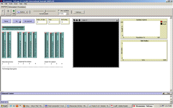Figure 4. The interface tab of NetLogo software platform.

3. Conceptual Validation

Despite the fact conceptual validation is very important there is little literature that addresses this issue (Robinson 2006). According to Heath (2009), the conceptual model forms the foundation of an ABM model; an invalid conceptual model indicates the model may not be an appropriate representation of reality.

3.1. The Analysis of Real Economic Systems

In this subsection we analyze the main features of economic systems implemented by the following types of society:

(i) Agrarian society is based on natural economy defined as a system where the majority of goods are produced for direct consumption (subsistence).

(ii) Industrial society implemented the process of social and economic change that transforms a human group from an agrarian type into an industrial one for the purpose of manufacturing goods not destined for direct consumption.

(iii) Green society generates a new type of economy called green economy that results in improved human well-being and social equity, with reducing environmental risks by implementing a new way of economic development based mostly on renewable resources.

3.2. Defining the Objective of Research and the Precise Task of the Model

Taking into account these three types of economic systems we defined the purpose of research as being the relation between technological progress and the distribution of wealth. The technological progress is implemented like a set of major changes in agricultural and industrial sectors. As we know both types of sectors use resources like water, food, coal, oil, gas, uranium, wind, sun, tides, and geothermal heat. To model the phenomenon of technological progress we conceived an agent-based artificial society described in Damaceanu (2011) as an evolutionary system that starts from the simplest type of economy (natural economy based only on water and food resources), continue with the industrial economy (that uses with maximum efficiency the resources of natural economy and discover nonrenewable resources such as coal, oil, gas, and uranium), and ends with the new economy (still using with maximum efficiency the resources of natural and industrial economies if they are available) based on renewable resources like wind, sun, tides, and geothermal heat. The technological progress is introduced in this model in linear way starting from agricultural technologies used in the case of natural economy, continuing with industrial technologies used for extracting nonrenewable resources in the following order coal, oil, gas, and uranium and ending with nonrenewable resources used in the following order wind, sun, tides, and geothermal heat.

The distribution of wealth is analyzed using Gini coefficient - see (Gini 1912). This coefficient is a measure of the inequality of a distribution, a value of 0 expressing total equality and a value of 1 maximal inequality. This index is defined as a ratio of the areas on the Lorenz curve diagram - see Figure 5.

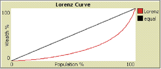Figure 5. Graphical description of Lorenz Curve.

3.3. Building the Conceptual Model

In section 2, we defined agent-based computational model (ACM) like a list of three arguments: the set of agents (A), the initializations (I) and the simulation specifications (R). The process of building the conceptual model can be defined like constructing the initial set of agents (A₀), setting the initial values of initializations (I₀) and specifying the initial values for simulation specifications (R₀) - see Figure 6, for a graphical description of the process. This figure shows us how the initial form of the ACM₀ enters in the phase of conceptual validation. If this validation fails the conceptual model is modified in a new form ACM₁ and the process is reiterated until conceptual validation is a success and the model become subject to operational validation.

Figure 6. The process of building the conceptual model.

3.4. Validation of Conceptual Model

The validation of conceptual model is a process that checks the integrity of all component elements of agent based model ACM_k divided in three major sets: the set of agents A_k, the set of initializations I_k and the set of simulation specifications R_k. In our case, because the model is developed in the frame of NetLogo software platform, we have the following set A_k = {O, T_i, P_xy}, where O is the observer agent that does not have a specific location - we can imagine it like an entity that observes the world composed by its sub-agents turtles T_i, and patches P_xy - see Figures 7-9.

Figure 7. The elements of Observer O.

Figure 8. The elements of turtles Ti.

Figure 9. The elements of patches Pxy.

The second set is I_k = (IO, IT_i, IP_xy), where IO are the initializations of O, where IT_i are the initializations of T_i and IP_xy are the initializations of P_xy - see Tables 1-3, and the third set is R_i = (rs, epw, epf, epc, epo, epg, epu, ewi, eps, ept, egh), where:

- rs is the seed of pseudorandom generator used by NetLogo. The seed may be any integer in the range supported by NetLogo (-9007199254740992 to 9007199254740992). In the context of scientific modeling, pseudo-random numbers are actually desirable. That is because it is very important for a scientific experiment to be reproducible;

- epw, epf = {0.1, 0.2, 0.3} are two control parameters called the efficiency of processing water and food;

- epc, epo, epg, epu = {0, 0.1, 0.2, 0.3} are four control parameters called the efficiency of processing coal, oil, gas and uranium;

- ewi, eps, ept, egh = {0, 0.1, 0.2, 0.3} are other four control parameters used in processing wind, sun, tides and geothermal heat.

Table 1. Initializations of O.

Table 2. Initializations of Ti.. Item Description i=a value from the set {1,2, ..., Tt} The identification number of the turtle Vi=a random value from the set {1, 2, ..., 15} A parameter that describes the vision of turtle how many patches ahead a turtle can see Li= a random value from the set {20, 21, ..., 80} Maximum age that a turtle can reach IMi A parameter that keeps the identification number of the mother IFi A parameter that keeps the identification number of the father Eit=Eit+(RWxyt·epw+ RFxyt·epf+RCxyt·epc+ ROxyt·epo+RGxyt·epg+ RUxyt··epu+RWIxyt·ewi+ RSxyt·eps, RTxyt·ept+RGHxyt·egh) A variable that keeps the value of energy processed from resources where epw, epf, epc, epo, epg, epu, ewi, eps, ept, egh are the parameters that measure the efficiency of processing water, food, coal, oil, gas, uranium, wind, sun, tides and geothermal heat. AGit=Li A variable that describes the age in years for every turtle WEit=0 A variable used to prevent two males from engaging the same female: 0 for no engaged and 1 for engaged IHit A variable used for the identification number of the husband MEit=0 A variable used to prevent two females from engaging the same male: 0 for no engaged and 1 for engaged IWit A variable used for the identification number of the wife PRit= A variable that has two possible values 0 for non pregnant woman and 1 otherwise PDit=1 A variable that keeps the value of pregnancy duration; this variable has a two possible values 0 (the initial value) and 1 when the turtle gives birth to a child.

Table 3. Initializations of Pxy.. Item Description x = a value from the set {-X, -X+1, ..., 0, 1, ..., X} Parameters that identify the horizontal coordinate of patch, where X=10 is the maximum x coordinate for patch y = a value from the {-Y, -Y+1, ..., 0, 1, ..., Y} Parameters that identify the vertical coordinate of patch, where Y=10 is the maximum y coordinate for patch RWxyt= a random value from the set {0, 1, 2, ..., 9} A variable owned by patch that keeps the value of water resources RFxyt= a random value from the set {0, 1, 2, ..., 9} A variable owned by patch that keeps the value of food resources RWIxyt= a random value from the set {0, 1, 2, ..., 9} A variable owned by patch that keeps the value of wind resources RSxyt= a random value from the set {0, 1, 2, ..., 9} A variable owned by patch that keeps the value of sun resources RTxyt= a random value from the set {0, 1, 2, ..., 9} A variable owned by patch that keeps the value of tides resources RGHxyt= a random value from the set {0, 1, 2, ..., 9} A variable owned by patch that keeps the value of geothermal heat resources RCxyt= a random value from the set {0, 1, 2, ..., 9} A variable owned by patch that keeps the value of coal resources ROxyt= a random value from the set {0, 1, 2, ..., 9} A variable owned by patch that keeps the value of oil resources RGxyt= a random value from the set {0, 1, 2, ..., 9} A variable owned by patch that keeps the value of gas resources RUxyt= a random value from the set {0, 1, 2, ..., 9} A variable owned by patch that keeps the value of uranium resources

4. Operational Validation

Operational validation can be defined as the transformation process of conceptual model in a model recognized by the software used (in our case NetLogo).

4.1. Transformation of Conceptual Model in a Computerized Model Using NetLogo Software Platform

In our case we used NetLogo 4.0.5 and, under these circumstances, we followed the cycles (see Figure 10):

- Cycle (1): modification of simulation specifications;

- Cycle (2): modification of parameters;

- Cycle (3): modification of initial values of variables;

- Cycle (4): modification of procedures;

- Cycle (5): development of new agents.

Figure 10. The cycles of operational validation of ACM.

Cycle (1) is the most frequent used. In this case, the researcher uses a previous created ACM or a new one in an incipient form, modifies the simulation specifications, runs the model, evaluates the simulation results and in function of these results takes the decision to apply one of the five available cycles.

Cycle (2) starts by changing the parameter values, running ACM, evaluation of results and in function of outcomes the researcher applies one of the five cycles.

Cycle (3) modifies the initial values of variables, runs ACM, evaluates the results and in function of these the researcher takes the decision to apply one of the five cycles.

Cycle (4) modify the set of procedures, runs the model and in function of results obtained after the evaluation the researcher apply one of the five cycles.

Cycle (5) develop new agents, run the model and in function of results the researcher takes the decision to apply one of five available cycles. This cycle usually creates new ACM.

The result of operational validation is the file 3Economies. nlogo available on NetLogo User Community Models site - see http://ccl.northwestern.edu/netlogo/models/community/3Economies.

4.2. The Operational Validation of Computerized Model

The operational validation is a technique that facilitates a more direct correspondence between the entities in the target system and the parts of the model that represent them (Edmonds 2001). This enhances the descriptive accuracy of the modeling process, but it can also create difficulties. Under these circumstances, almost every operational validation of agent-based models may contain bugs defined as code that does something different in comparison with what you expected (Gilbert 2007). As Axelrod underlines, you have to work hard to confirm that the operational validation is really valid (Axelrod 1997). In addition, Axtell and Epstein state that “the robustness” of macrostructures to perturbations in individual agent performances is specific to agent-based models and makes very hard to identify bugs (Axtell and Epstein 1994).

Computer experiments can be seen as a branch of applied statistics, because the user must take into account the next sources of uncertainty:

(i) First, the models may contain parameters whose values are not certain;

(ii) Second, the models themselves are imperfect representations of the studied system;

(iii) Third, data collected from the system that might be used to calibrate the models are imperfectly measured.

Taking into consideration the evolution in time of economy described in Figure 11, we will do 9 computer experiments described in Table 4.

Figure 11. The evolution in time of economy.

Table 4. Description of computer experiments. Name Description E1 This experiment is called Agricultural Revolution and has 9 runs that describes a economy based on water and food converted in energy with the following control parameters rs = 0, epw = {0.1, 0.2., 0.3}, and epf = {0.1, 0.2, 0.3}. E2 This experiment is called Industrial Revolution 1 and has 3 runs that describes a economy based on water, food, and coal converted in energy with the following control parameters rs = 0, epw = 0.3, epf = 0.3, and epc = {0.1, 0.2, 0.3} E3 This experiment is called Industrial Revolution 2 and has 3 runs that describes a economy based on water, food, coal, and oil converted in energy with the following control parameters rs = 0, epw = 0.3, epf = 0.3, and epc = 0.3, and epo = {0.1, 0.2, 0.3} E4 This experiment is called Industrial Revolution 3 and has 3 runs that describes a economy based on water, food, coal, oil, and gas converted in energy with the following parameters rs = 0, epw = 0.3, epf = 0.3, and epc = 0.3, and epo = 0.3, and epg = {0.1, 0.2, 0.3} E5 This experiment is called Industrial Revolution 4 and has 3 runs that describes a economy based on water, food, coal, oil, gas, uranium converted in energy with the following parameters rs = 0, epf = 0.3, epw = 0.3, and epc = 0.3, and epo = 0.3, epg = 0.3, and epu = {0.1, 0.2, 0.3} E6 This experiment is called Green Revolution 1 based on water, food, coal, oil, gas, uranium, and wind converted in energy and has 3 runs with the following parameters rs = 0, epf = 0.3, epw = 0.3, and epc = 0.3, and epo = 0.3, epg = 0.3, and epu = 0.3, and ewi = {0.1, 0.2, 0.3} E7 This experiment is called Green Revolution 2 based on water, food, coal, oil, gas, uranium, wind, and sun and has 3 runs with the following parameters rs = 0, epf = 0.3, epw = 0.3, and epc = 0.3, and epo = 0.3, epg = 0.3, and epu = 0.3, and ewi = 0.3, and eps = {0.1, 0.2, and 0.3}. E8 This experiment is called Green Revolution 3 based on water, food, coal, oil, gas, uranium, wind, sun, and tides and has 3 runs with the following parameters rs = 0, epf = 0.3, epw = 0.3, and epc = 0.3, and epo = 0.3, epg = 0.3, and epu = 0.3, and ewi = 0.3, and eps = 0.3, and ept = {0.1, 0.2, 0.3} E9 This experiment is called Green Revolution 4 based on water, food, coal, oil, gas, uranium, wind, sun, tides, and geothermal heat and has 3 runs with the following parameters rs = 0, epf = 0.3, epw = 0.3, and epc = 0.3, and epo = 0.3, epg = 0.3, and epu = 0.3, and epw = 0.3, and eps = 0.3, and ept = 0.3, and egh = {0.1, 0.2, 0.3}.

5. Conclusions

Based on data obtained after running the nine computer experiments, we computed the average value of Gini coefficient and using these averages we can describe the evolution of mean value of Gini coefficient in the case of experiments E1-E9 - see Table 5 and Figure 12.

Table 5. The evolution of average value of Gini coefficient in the case of experiments E1-E9. Experiment Average value of Gini coefficient obtained during runs Mean value of Gini coefficient E1 run 1 0.525654612 0.540133744 run 2 0.537615676 run 3 0.538179805 run 4 0.537846548 run 5 0.542855952 run 6 0.548644241 run 7 0.53638687 run 8 0.544669638 run 9 0.549350355 E2 run 1 0.545503647 0.546935308 run 2 0.548006924 run 3 0.547295354 E3 run 1 0.546807708 0.545424903 run 2 0.542766655 run 3 0.546700346 E4 run 1 0.546488227 0.546123743 run 2 0.54449901 run 3 0.547383991 E5 run 1 0.547190046 0.54727205 run 2 0.545231192 run 3 0.549394911 E6 run 1 0.549698197 0.549710616 run 2 0.550984873 run 3 0.550431387 E7 run 1 0.553987988 0.556033016 run 2 0.557564208 run 3 0.556546854 E8 run 1 0.563820991 0.563476579 run 2 0.562037514 run 3 0.564571232 E9 run 1 0.564478662 0.564196023 run 2 0.564292289 run 3 0.563817118

Figure 12 shows us that the technological progress has a negative influence on wealth equality measured by Gini coefficient and this is explained by the heterogeneity of turtles' population Ti given by their variable vision Vi. On the other hand, technological progress has a positive influence on number of turtles but the distribution of wealth become more and more unequal because fewer turtles are "rich" and many others are "poor".

Figure 12. The evolution of mean value of Gini coefficient in the case of experiments E1-E9.