1. Introduction

Systems that utilize networks for communication between industrial systems and controllers are called network control systems (NCS) and by this way reduction of wiring and ease of maintenance are achieved [1–4]. Viewed from a different perspective, systems that consist of sensors, actuators, controllers and supervisory computers which communicate between each other over a computer network are also called NCS [1–7]. However an appropriate SOA technology for NCS must provide a bounded transmission delay and interoperability between different components of the NCS. Several efforts have been made for embedding a SOA technology into industrial control loops but none of them can provide both the desired characteristics [8–10].

It is now common in industrial control to use computer networks for passing measurements collected from sensors to the controllers, that is, the computing facilities which execute the control algorithms and transmitting the commands produced by the controllers to the actuators which adjust the values of the controlled variables [2,4,11]. Furthermore, a second level of computer networks is used for the communication of the controllers with higher level computers which perform operations management and supervisory or cell control [2,11–15]. The uses of computer networks in industrial control applications has the benefits of reduced wiring and eases of maintenance and are usually build with special architectures and protocols which provide a bounded transmission delay [2,8–15]. However they suffer from high hardware and software cost, and the inability to be linked directly to ordinary IP networks, build around the IEEE 802.3 Ethernet technology which would allow them to communicate with ordinary computing facilities available off-the self at low cost or are used an industrial organization [16] for office or computer-aided design/computer-aided engineering (CAD/CAE) functions. Such facilities can offer enhanced computing power, sophisticated graphics and mathematical processing software. The recent advances on service oriented architectures (SOA) for networks [16] build again over IP networks and offered in the form of standardized off the shell solutions make even more attractive the replacement of the special high cost architectures of the NCS with such architectures. SOA architectures offer high degree of flexibility, interoperability, ease of use and application development over the IP protocol, and complete language and platform independency. However, as it might be expected, it offers all these advantages at the cost of higher communication overhead. To use it in NCS there must be found ways of implementing these concepts at lower communication costs so the time limits imposed on the exchange of information in a NCS must be met. To this end a protocol stack was developed to embed the SOA technology, based on web services (WS), into sensors and actuators. It is called the device profile for web services (DPWS) [17] based on a SOA implementation with reduced bandwidth requirements. However, to extend the SOA concepts to advanced control strategies, such as nonlinear adaptive model predictive control (NAMPC), a further reduction in the bandwidth requirements is needed. [2,11,12,18].

The transmission time for the data packets introduces network-induced delays to NCSs, which are well known to degrade the performance of the control systems [2,11–14]. There are two types of network-induced delays according to where they occur, namely [2,11–14]: (i) τ_sc is network-induced delay from the sensor to the controller, that is, backward channel delay; and (ii) τ_ca is network-induced delay from the controller to the actuator, that is, forward channel delay. These two types of network-induced delays may have different characteristics; and in most cases, however, these delays are not treated separately and only the round trip delay is of interest [2,11–14].

According to these types of communication networks being used in NCSs, the characteristics of the network-induced delay vary as follows [2,11–14]: (i) Cyclic service networks (e.g., Toking-Ring and Toking-Bus) are bounded delays which can be regarded as constant for most occasions; (ii) Random access networks (e.g., Ethernet and CAN) are random and unbounded delays; and (iii) Priority order networks (e.g., DeviceNet) are bounded delays for the data packets with higher priority and unbounded delays for those with lower priority.

As it is demonstrated in this work such a reduction can be achieved if a proposed new computer network architecture for NCSs is used. In this architecture the DPWS technology is modified by introducing a new format for the exchange of messages in the network and is combined with the use of switched Ethernet. In this way an overall bounded transmission delay among the sensing and actuating devices is achieved. The performance of this network has been assessed in an industrial case study which involved the implementation of an adaptive predictive control algorithm for the control of a fluidized bed furnace reactor (FBFR) of the steam deactivation unit of a fluid catalytic cracking (FCC) pilot plant.

The paper is structured as follows. An overview of the proposed computer network as well as the protocol architecture that it is based on is presented in Section 2. The utilized SOA technology used by the components of this network is given in Section 3. The new control algorithm is explained in Section 4. The implementation of the algorithm over the proposed computer network for the control of the FBFR process is explained in Section 5. In the same Section simulation results are presented. Section 6 concludes the paper and highlights its major contributions.

2. Description of the Network Control System (NCS)

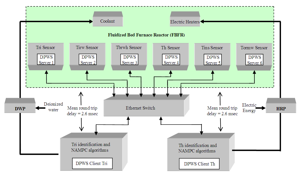
The proposed architecture for the NCS used in this work is shown in Figure 1. Every transmission medium in this system constitutes the proposed SOA based on DPWS which consists of two levels: the device and the cell levels as shown in Figure 1. The transmission medium between any of these two levels of the automation system is considered to have the switched Ethernet architecture. In Figure 1, q is the number of sensors defining the outputs of a process and p is the number of actuators denoting the control inputs to the process. The control system (identification and control algorithms) is located at the cell level while the q sensors and p actuators are at the device level. The plant and enterprise levels comprise the enterprise resource planning system, management and supervisory operations as well as the monitoring and control of an industrial process.

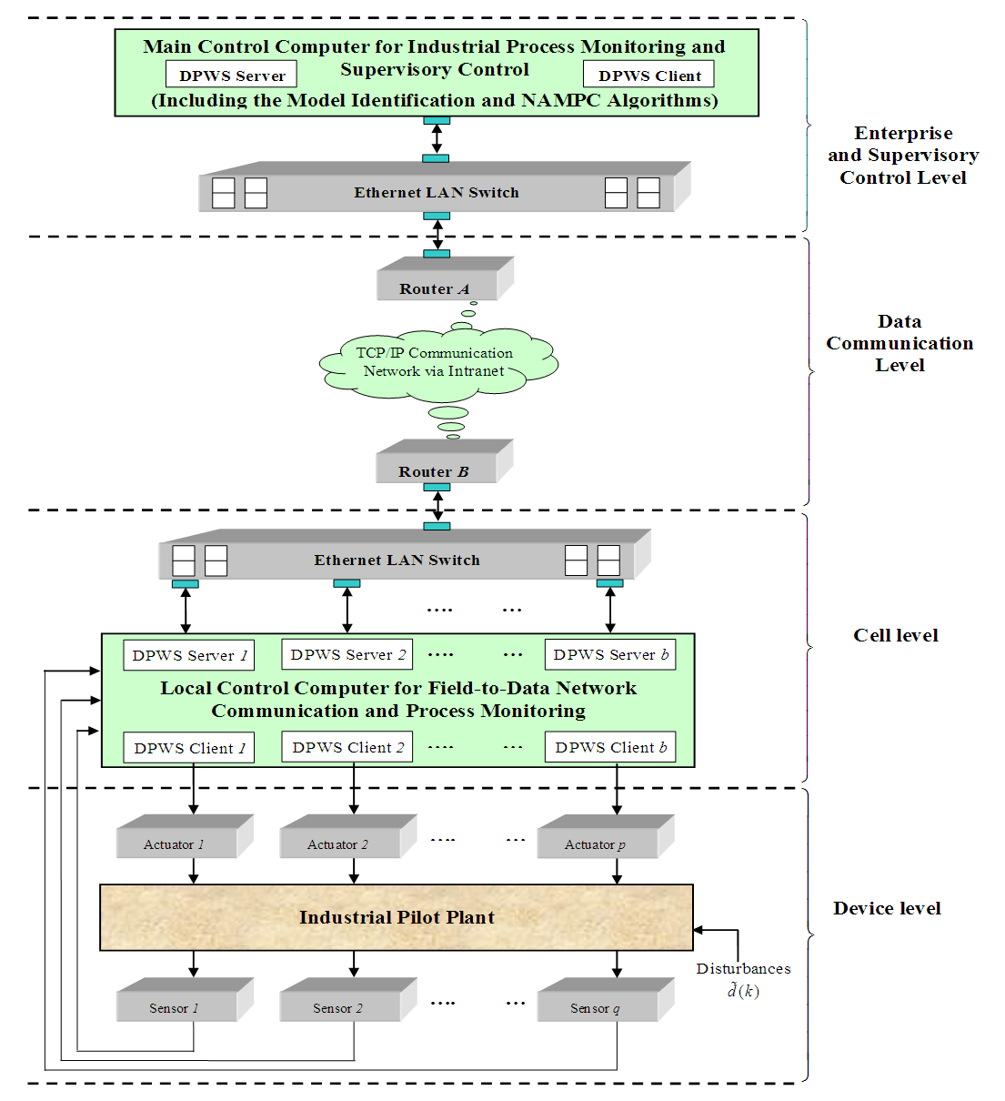Figure 1. The proposed four-level network control system (NCS) architecture based on hierarchical structure

Summarizing the function of the basic communication devices, the hub connects nodes together, a switch determines where data goes, a router determines what kind of data goes in or out, and a firewall blocks malicious data traffic [2,14,15]. In fact, switches operate on Layer 2 frames while routers operate on Layer 3 packets [13]. These devices can be combined elegantly to construct a network that sends data exactly to where and to whom it should go and denies malicious data from ever landing on the network [2,13–15]. In the following sub-section, how the proposed NCS is industrial network control system offers bounded transmission delay is presented.

2.1. Switched Ethernet Architecture and SOA Technologies

2.1.1. The Architecture of the Switched Ethernet Based on Local Area Network (LAN)

Ethernet specification defines a number of wiring and signaling standards for the physical layer of the open systems interconnection (OSI) networking model as well as a media access control (MAC) algorithm and a common addressing format at the data link layer (DLL). However, it is impossible to guarantee a bounded message transmission time mostly due to its weakness to handle collisions.

In switched Ethernet data is transmitted and received on different wires and the hub is replaced by an Ethernet switch. The carrier sense multiple access with collision detection (CSMA/CD) MAC protocol is no longer used in switched Ethernet. The switch regenerates the information and forwards it only to the port on which the destination is attached. It complies with the IEEE 802.3 MAC protocol when relaying the frames and creates different collision domain per switch port whereas in the hubs all the nodes have to share the bandwidth of a half-duplex connection. If a frame is already being transmitted on the output port, the newly received frame is queued and will be transmitted again when the medium becomes idle. In addition, all cables are point to point, from one station to a switch and vice versa. So it is allowed to have dedicated bandwidth on each point to point connection with every node running in a full duplex mode with no collisions. This characteristic renders the switched Ethernet appropriate for industrial applications where the response time is a crucial matter. Furthermore, apart from the cases in which overflows occur in the switches, transmission bounds can be predicted [2,11,12,19]. However, overflows may occur if for example the combined traffic destined to the same destination may exceed the capacity of the link between the switch and destination. The excess traffic accumulates in the switch until its output buffer overflows. In such a case no strict bound can be considered on the transmission delay.

2.1.2. SOA Technologies

Nowadays, service-oriented architecture (SOA) has become the state of the art solution for implementing autonomous and interoperable systems as it provides web-based and modular implementation of complex and distributed software systems [20]. The interoperability at the application level that it offers due to its loosely coupled nature renders it a desirable element when developing information and communication technology (ICT) systems.

Several device level SOA technologies have been proposed, most notably Jini [21], universal plug-n-play (UPnP) [22] and device profile for web services (DPWS) [17].

2.1.2.1. The Jini Technology

Jini offers the ability to register, discover, and use services [21]. However is highly rooted in Java and therefore is not designed for completely language and platform independency.

2.1.2.2. The UPnP Technology

The UPnP architecture leverages Internet and Web technologies including Internet protocol (IP), transfer control protocol (TCP), user datagram protocol (UDP), hypertext transfer protocol (HTTP), simple object access protocol (SOAP), and extensible markup language (XML). However, it is not fully compatible with web services (WS) technology. Furthermore it uses specific protocols for discovery and event notification purposes.

2.1.2.3. The DPWS Technology

The DPWS has adopted WSs technology and therefore it provides plug-n-play connectivity and completely language and platform independency [23,24]. For these reasons, the DPWS is the preferred implementation vehicle for SOA technology in the present study.

DPWS utilizes Internet and web technologies including IP, TCP, UDP, HTTP, simple object access protocol (SOAP), extensible markup language (XML) as well as web services description language (WSDL) 1.1. As it is documented in [20], the core WSs standards are the following: WSDL, XML Schema, SOAP, WS-Addressing, WS-Policy, WS-MetadataExchange and WS-Security. Apart from the standard core WSs, DPWS adds WS-Discovery for WS discovery and WS-Eventing for subscription mechanisms. A detailed description of these protocols can be found in [17,23–25].

2.2. The Utilized Service-Oriented Architecture (SOA) Technology

Recently, SOA has become the state of the art solution for implementing autonomous and interoperable systems [16]. Several device level SOA technologies have been proposed, most notably DPWS [17], Jini [21] and universal plug-n-play (UPnP) [22]. Jini is highly rooted in Java while UPnP is not compatible with WS technology. Therefore, they are not designed for complete language and platform independency. On the other hand, the DPWS has adopted WSs technology [23–25]. For these reasons, the DPWS is the preferred implementation vehicle for SOA technology in the present study.

DPWS utilizes Internet and web technologies including IP, TCP, UDP, HTTP, simple object access protocol (SOAP), extensible markup language (XML) as well as web services description language (WSDL) 1.1. As reported by Jammes and Smit, the core WSs standards are the following: WSDL, XML Schema, SOAP, WS-Addressing, WS-Policy, WS-MetadataExchange and WS-Security [16]. Apart from the standard core WSs, DPWS adds WS-Discovery for WSs discovery and WS-Eventing for subscription mechanisms. A detailed description of these protocols can be found in [2,13–17].

In order to adopt the benefits of the DPWS, all the components in the proposed computer network conforms to the DPWS specification implemented on top of switched Ethernet architecture. The sensors and actuators have DPWS server interfaces and so are DPWS servers, while the control system has DPWS client interface and therefore is DPWS client as it is shown in Figure 1. It has been argued that the device-level SOA interaction patterns can be categorized according to six levels of functionality: addressing, discovery, description, control, eventing and presentation [23–25]. After the discovery phase where the DPWS client has discovered the sensors and actuators, it subscribes to the events of them by publishing the required sampling period using the eventing level interaction. Every DPWS server assumes that whenever this time expires, there is a change in its state and so it informs the DPWS client with the new values using the WS-Eventing protocol. Moreover, the DPWS client informs the actuators with the new control signals as soon as the control algorithms have finished their execution, by using the control level interaction. The network can be considered real-time only if the worst case overall control loop delay is bounded and less than the sampling period.

However the current DPWS technology suffers from the high utilization of network bandwidth especially when it is used on top of non-deterministic protocols such as Ethernet as it exchanges DPWS messages which are XML documents [18]. Therefore in this study a compression technique is proposed for reducing the size of these documents. This compression technique is called indiscriminate application specific format technique (IASFT) and renders the DPWS suitable for online advanced control of industrial processes with sampling time similar to those of the FBFR even if the Ethernet technology is used as investigated in Section 5.

2.3. The Indiscriminate Application Specific Format Technique (IASFT)

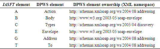
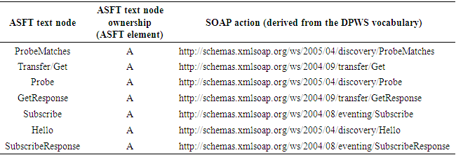
It is well known that the performance bottleneck of current WSs technology is the need for continuously parsing XML documents whose data volume is high. However their usage is a necessity when considering application level interoperability issues. The benefits of using XML documents can be found in [26]. Binary-based encodings [27] such as the efficient XML interchange (EXI) format which seems to be the most commonly used overcomes this barrier by defining a compact representation of XML documents in a binary format. But this format does not conform to the XML specification. Arguably, in a SOA-based system it is extremely important that there are no standards applied that limit the use of the service to only a specific platform. By introducing the binary XML this characteristic is being omitted. Moreover by utilizing binary XML encodings, the simplicity of using the human readable XML documents is lost and third-party tools are needed in order to transform them back to a human readable form. Finally as it is documented in [28], XML documents are faster to read than the equivalent binary files in standard applications due to XML hierarchical structure.

Bearing all these facts in mind a technique is proposed for reducing the message size of XML documents without prohibiting the usage of XML and other WSs standards. This compression technique is called IASFT. The IASFT mechanism transforms DPWS messages to IASFT messages and vice versa according to the IASFT specification. This mechanism is placed between the core WSs standards of the DPWS and the transport protocols on every component in the proposed computer network. When these components create DPWS messages, the IASFT mechanism transforms them to the equivalent IASFT messages and sends them to the network using the transport protocols. On the other hand, when a component receives IASFT messages, the IASFT mechanism transforms them to the equivalent DPWS messages before it forwards them to the DPWS WSs standards. Before continuing with the description of the IASFT, it must be mentioned the connection between an XML document, an XML application, an XML schema and a developed application. XML application is a specific XML vocabulary that contains particular elements and attributes that limit the flexible rules of XML. Based on the application environment, different XML applications are developed. According to these applications, appropriate XML documents are constructed that describe particular events occurred in the application environment. Nevertheless these XML documents must be validated against to the XML schema that is produced based on the developed XML application too. Lastly, the developed application is designed to manipulate the validated XML documents and extract information according to the XML application.

In the proposed computer network a new XML application is invented for describing the capabilities of the devices based on the IASFT format. This new application aims to describe the DPWS application by using the new format. This is feasible by utilizing bindings that associate DPWS elements which are elements used by the DPWS application to IASFT elements which are elements used by the new format of the IASFT application. Some of the IASFT elements as well as their bindings to DPWS elements are listed in Table 1.

Table 1. Some IASFT elements bindings to specific DPWS elements

The basic building principles of the IASFT are summarized as follows:

1). IASFT messages are XML documents. Moreover DPWS messages have the structure of SOAP envelope which consists of header and body elements. This structure is maintained. IASFT messages consist of header and body IASFT elements. Therefore the communication remains independent of the message content;

2). The IASFT uses extensible stylesheet language transformations (XSLT) version 2.0 [29] for describing the rules of transformations. This is accomplished by using XSLT stylesheets which actually describe how documents in DPWS format are converted to documents in IASFT format and vice versa. These stylesheets consist of template rules that contain XSLT instructions which are applied to the selected nodes and are based on the IASFT elements bindings;

3). The name of every element in IASFT messages must have UTF-8 encoding style as implied by the XML specification [11,13–15,26] and must have the minimum length. This means that the names are identified by only one character;

4). Start-tags must be matched by end-tags;

5). In order to maintain the independency and the interoperability feature of XML documents and in the meantime associate the IASFT messages with the equivalent DPWS messages, every IASFT message has the default namespace “http://iasft” in its envelope root element. This indicates that all the elements in the current XML document are affiliated with this namespace. Therefore they have particular semantics which is their association with various DPWS elements as listed in Table 1. By this way the DPWS standards are not distorted;

6). Using the IASFT elements bindings, the IASFT mechanism can transform DPWS messages to IASFT messages with the same semantics and vice versa;

7). No namespaces are used in IASFT messages except from the default namespace which has already unambiguously qualified all the IASFT elements;

8). Only the namespaces used in “Types” elements for discovery purposes and target namespace declarations in DPWS messages are used in IASFT messages. However they are inserted as text nodes within the text of the corresponding IASFT elements;

9). No attributes are used in IASFT messages. Instead they are inserted as text nodes within the text of the corresponding IASFT elements. When the IASFT mechanism transforms back an IASFT message to DPWS message, it indicates these text nodes as attributes of the corresponding DPWS elements;

10). The text nodes of the “Action” elements in DPWS messages which identify the semantics implied by SOAP action of the messages are substituted by the equivalent ASFT text nodes which are listed in Table 2. There is no need to use a full uniform resource identifier (URI) field for describing the SOAP action as the developed application by the IASFT is able to understand the IASFT text nodes. These are associated with specific SOAP actions derived from the DPWS vocabulary. These associations are listed in Table 2. Using these bindings the IASFT mechanism can transform a SOAP action accepted by the new developed IASFT application to a SOAP action from the DPWS vocabulary and vice versa;

11). The “MessageID” element is used by the DPWS in order for every DPWS message to be uniquely identified in a network. However, during TCP interactions in the proposed computer network every exchanged message can be uniquely identified by the target IP address plus the target port number plus the TCP sequence number assigned to it. During UDP communications which take place only in discovery interaction in a DPWS-based network, every exchanged message can be easily identified by its source IP address plus the source port number plus the scopes and type information embedded in it as WS-Discovery protocol implies. So IASFT deletes the “MessageID” elements as well as its text node; and

12). DPWS allows the child elements of the SOAP body element in DPWS WS-Eventing notification messages to be unambiguously named by being qualified with a target namespace. IASFT notification messages do not use this namespace and so is deleted by the IASFT. The child element of envelope’s body in the IASFT notification message is associated with the endpoint reference address which is a transport address located in header’s child IASFT element “T”. This address is unique as it is generated for this specific interaction. It points to the subscription-end recipient. Therefore in IASFT messages the envelope’s body child element is already unambiguously qualified. Moreover the target namespace is already published to the client during the metadata exchanges [17]. The aforementioned characteristics alleviate the need of the target namespace in IASFT notification messages.

Table 2. IASFT text nodes bindings to specific SOAP actions

The seventh, eighth and ninth building principles enables the IASFT messages to be considered as pure XML documents. Therefore, the XML-remote procedure calls (RPC) is to manipulate pure XML documents instead of the heavy SOAP engine which is able to process complicated XML documents [30].

In Figure 2, it is shown how the IASFT mechanism transforms a DPWS WS-Eventing notification message to the equivalent IASFT event notification message. For example the “Envelope” element from the DPWS message that has the “soap” prefix which is bound to a specific namespace is transformed to the “E” element according to the bindings expressed in Table 1. Also the target namespace used for qualifying the child elements of the SOAP body element in DPWS message is deleted in the IASFT message.

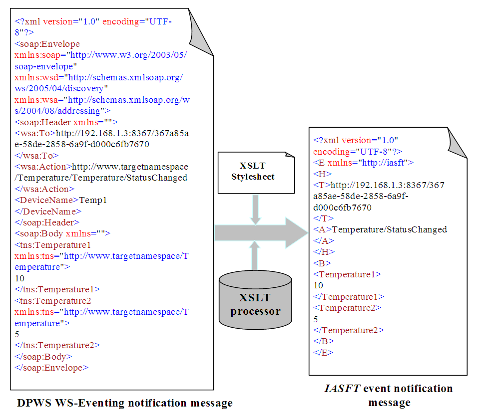Figure 2. DPWS WS-Eventing notification message transformation according to the IASFT specification

From the IASFT building principles it is clear that the IASFT messages are considered XML documents as they satisfy the document production in the Backus-Naur form (BNF) grammar and adhere to the well-formedness constraints described in [26].

2.4. Bounded Transmission Delay

Although, studies have proposed some industrial solutions for satisfying real-time requirements with respect to bounded transmission delay; but however, these solutions suffer from the high hardware and software cost [8,9]. On the contrary, a simple and accepted solution for connecting devices within a NCS has been reported [10]. The switched Ethernet is chosen as the transmission medium. This medium eliminates frame collisions, uses inexpensive and widely accepted technology as it is compatible with IEEE 802.3 technology and provides a predicted transmission bound as long as overflow events do not occur in the switches [2,10–15,19]. It has been documented in several reports that switched Ethernet architecture can be used throughout the architecture of an automation system [2,10–14]. In this way interoperability is provided at the network interface level, i.e. devices use the same medium access control (MAC) and physical layer (PHY) interfaces for connecting with each other.

The proposed computer network uses the same architecture and the worst case transmission delay of a data frame transmitted from the device level to the control system is observed when all the sensors and actuators transmit data simultaneously. This delay can be defined as follows:

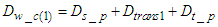(1)

where is the processing transmission delay at the sensors and actuators, is the transmission delay, i.e. the delay in queue plus the delay in the network, and is the frame reception delay at the control system. When a TCP connection is established, its delay must also be taken into account. This connection is established by the exchange of a CONNECTION-REQUEST message and a CONNECTION-ACCEPTED segment as it is documented in [31]. Again the worst case TCP connection establishment delay is observed when all the devices that are located at the device level request such a connection simultaneously. Therefore the worst case CONNECTION-REQUEST delay from the device level to control system is:

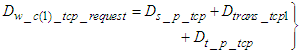(2)

where is the TCP processing transmission delay at the sensors and actuators while is TCP processing reception delay at the control system. These delays correspond to the flow of data from the transport layer to the PHY layer and vice versa. is the transmission delay of the TCP request segment transmitted from the device level to the control system. The worst case CONNECTION-ACCEPTED delay which is denoted as is the delay experienced when the last CONNECTION-ACCEPTED segment is sent by the control system to device level and is the same with . Now, the worst case transmission delay that a TCP data segment experiences when it is transmitted from the device level to the control system is defined by using Equations (1) and (2) as:

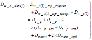(3)

Let be the overall processing delay that the TCP data segment experiences when it is sent from the device level to the control system and 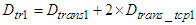be the overall transmission delay that a TCP data segment experiences for the same path. Then Equation (3) is formed as:

(4)

The worst case transmission delay of a frame transmitted by the control system to the device level is the delay that the last frame in the control system queue experiences and can be calculated as:

where is the computational time that the identification and control algorithms need for computing the control input signals to the process, is the processing transmission delay at the control system and is the frame reception delay at the device level and is the transmission delay a frame sent from the control system to the device level. When a TCP connection is established, it must be taken into account the TCP connection establishment delay too. Following the same way with the one presented previously, the worst case transmission delay that a TCP data segment experiences sent from the control system to the device level is defined as:

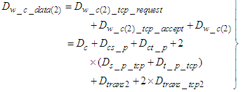(5)

where is the transmission delay of the TCP request segment transmitted from control system to the device level. Let be the overall processing delay a TCP data segment experiences due to transmission by the control system to the device level and let 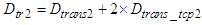be the overall transmission delay a TCP data segment experiences for the same path [2,11,13,14]. Then Equation (5) is formed as:

(6)

The combination of Equations (4) and (6) determines the worst case overall control loop delay of the proposed computer network:

(7)

From the above it is understood that the proposed computer network can be used in an industrial application if data is transmitted with TCP connection and the real time requirement is below the as this is the bounded delay that it can offer as long as there are no overflow events in the switches.

2.5. Interoperability at the Application Level

Up to this point, it has been assumed that interoperability is provided at the network interface level by the proposed SOA based on DPWS. In order to enable every component in the proposed NCS to interact with any other node regardless the language or implementation platform, the interoperability feature must be provided at the application level too. Therefore the DPWS must be adopted by all the components of the proposed NCS based on SOA computer network based on DPWS as it provides the aforementioned interoperability as discussed in Section 2.1.

As discussed in Section 2.2, all the components in the proposed SOA computer network based on DPWS conform to the DPWS specification implemented on top of switched Ethernet architecture as shown in Figure 1.

Since in this network all the components conform to the DPWS implemented on top of Ethernet specification, all the exchanged messages have the SOAP structure. The structures that all the exchanged messages have in the proposed NCS are illustrated in Figure 3. The root element of a SOAP message is the Envelope. It encloses one or two child elements: an optional Header and a Body. The Header element carries information that does not directly belong to the payload of the message, while the Body element contains the actual payload of the message. Finally, a namespace is used in the XML representation for using unambiguous data formats [13,14].

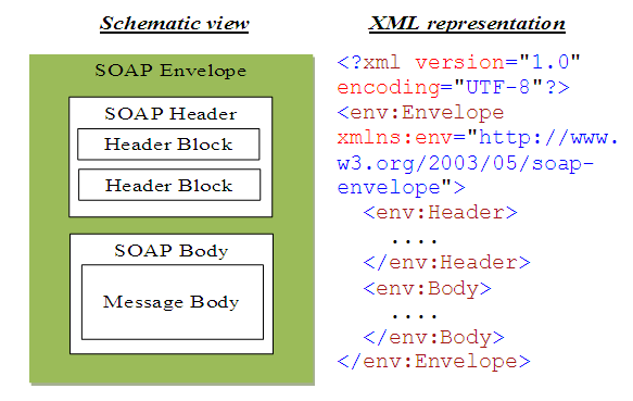Figure 3. Structure of a SOAP message

3. The FBFR Process Description

The FBFR is a sub-unit of a pilot plant scale steam deactivation unit (SDU) shown in Figure 4. The SDU is a pilot plant fitted with automated controls for temperature and gas supply switching. The operation is coordinated by a state of the art industrial control system and software. Three gas lines each consisting of filter, pressure regulator, pressure indicator and check valve are fed to a single mass flow controller. An on–off solenoid valve manages the flow of each line. An accurate deionized water pump (DWP) supplies the water that is required for steam generation through the upper part of the line entering the FBFR (see Figure 4). The FBFR is a cyclic propylene steaming unit that is used to prepare catalysts for evaluation in FCC pilot plant.

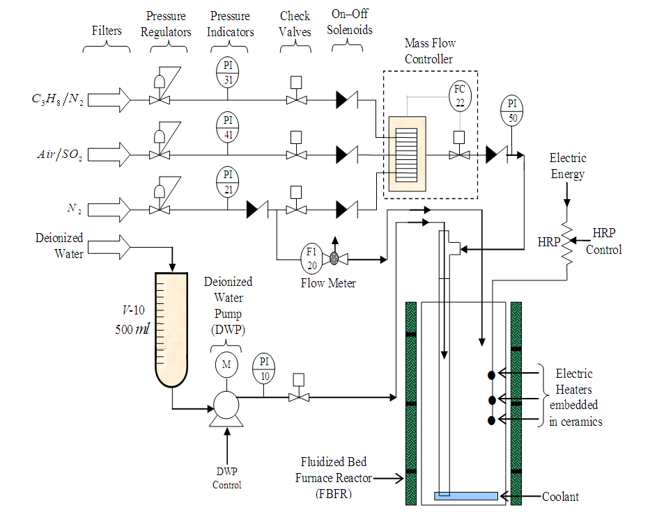Figure 4. Simplified diagram of the steam deactivation unit (SDU) of the FCC pilot plant

The FBFR considers heat transfer in the radial direction for a structure consisting of successive cylindrical layers as shown in Figure 5. Electric heaters are embedded in ceramic material in the heater section to generate the necessary heat for the process. The heaters are controlled by high resistance potentiometer (HRP). Heat is then transported in the radial direction towards the centre of the reactor and the insulator section. The complete FBFR process description and the dynamic behaviour of the temperature expressed as a set of partial differential equations are given and described in [32–35].

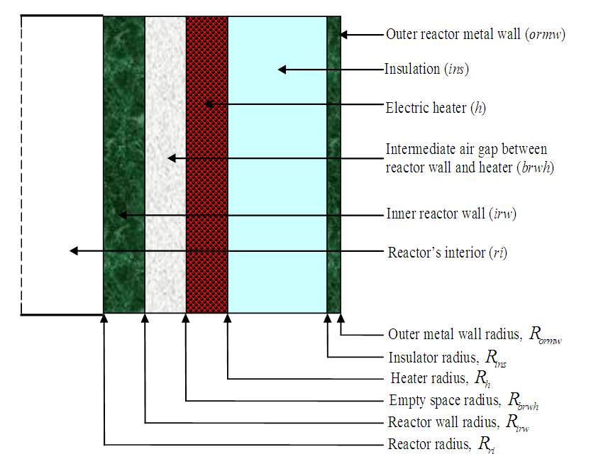Figure 5. Schematic of the vertical cross-section of the cylindrical fluidized bed furnace reactor (FBFR) of the SDU

The deactivation involves the exposure of catalyst to streams containing steam, propylene, SO₂, and nitrogen for a specified number of cycles at high temperature of up to 1060°K during initial heat up. The most essential element in the cyclic propylene steam deactivation procedure involves the tight control of the temperature inside the reactor and that of the heater not exceeding 860°K and 1040°K respectively. In a previous work [35], nonlinear MPC with N_u = _Np = 40 and proportional-integral-derivative (PID) controllers gave undesirable temperature overshoots of 281 °K and 288 °K respectively using the FBFR process mathematical model with a sampling time of 2 minutes.

4. The Neural Network Model Identification and Neural Network-Based Control Schemes

4.1. The FBFR Neural Network Model Identification Scheme

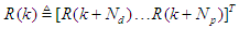
Assuming that at time , the FBFR process can be represented by as a p-input q-output nonlinear discrete-time system with disturbance term by the following nonlinear autoregressive moving average with exogenous inputs (NARMAX) model [32–34]:

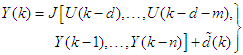(8)

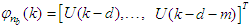
where is a nonlinear function of its arguments, and 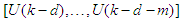are the past input vector, 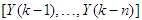are the past output vector, is the current output, and are the number of past inputs and outputs respectively that define the order of the system, and is time delay. The predictor form of Equation (8) based on the information up to time can be expressed as [32–34]:

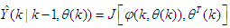(9)

where is the regression (state) vector, and is an unknown parameter vector which must be selected such that 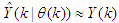, is the error between Equations (8) and (9) defined as:

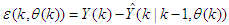(10)

Let a set of input-output data pair obtained from prior system operation over NT period of time be defined as:

(11)

where is the sampling time of the system outputs. Then, the minimization of Equation (10) can be stated as follows:

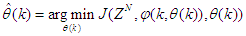(12)

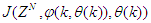where is formulated as a mean square error (MSE) type cost function which can be stated as:

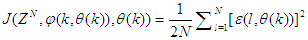(13)

The inclusion of as an argument in is to account for the desired model dependency on. Thus, given an initial small random value of , and Equation (11), the model identification problem reduces to the minimization of Equation (12) to obtain .

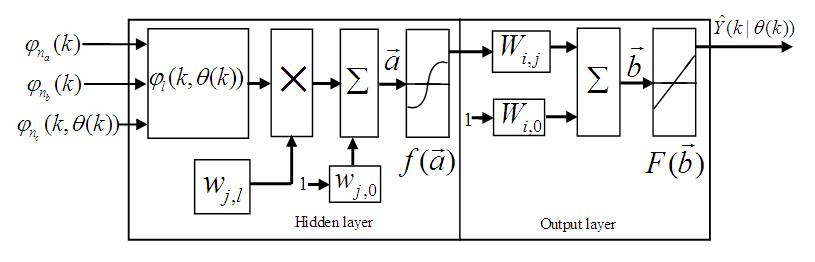
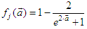
The minimization of Equation (12) is approached by considering as a neural network model. The complete NN model identification scheme based on the teacher-forcing method is illustrated in Figure 6 [34]. According to this scheme, the validated mathematical model of the FBFR process is placed in parallel with its NNARMAX model (in the dashed box) where the TDL (tapped delay line memory) are used to store temporal NN input information. The architecture of the “Neural Network Model” of Figure 6 is a dynamic feedforward NN (DFNN) shown in Figure 7. The inputs to the DFNN model of Figure 7 are 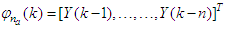, and which are concatenated into as shown in Figure 7. The output of the NN model of Figure 6 in terms of the network parameters of Figure 7 is given as:

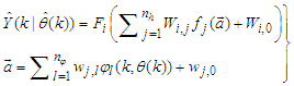(14)

where and are the number of hidden neurons and number of regressors respectively; i is the number of outputs, and are the hidden and output weights respectively; and are the hidden and output biases; is a linear activation function for the output layer and is an hyperbolic tangent activation function for the hidden layer defined here as:

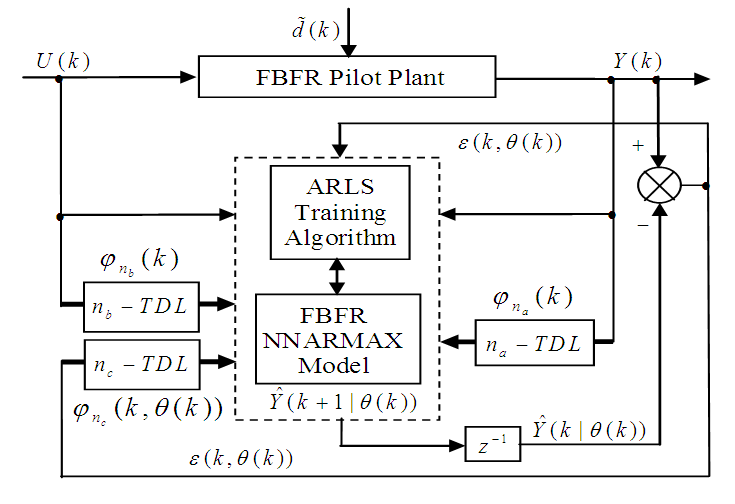Figure 6. The FBFR NNARMAX model identification scheme using ARLS training algorithm

Figure 7. Architecture of the dynamic feedforward NN (DFNN) model

(15)

The term “bias” is a weight acting on the input and clamped to 1. Here, is a collection of all network weights and biases in Equation (14) in term of the matrices and . Equation (14) is here referred to as NN NARMAX (NNARMAX) model predictor for simplicity.

The in Equation (8) is usually unknown but can be estimated as a covariance noise matrix using 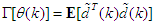with an iterative algorithm described in [32–34]. Thus, using, Equation (13) becomes:

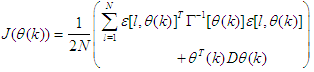(16)

where the second term in Equation (16) is the regularization (weight decay) term which has been introduced to reduce modeling errors, improve the robustness and performance of the training algorithms [34]. is a penalty norm and also removes ill-conditioning, where is an identity matrix, and are the weight decay values for the input-to-hidden and hidden-to-output layers respectively. Note that both and are adjusted simultaneously with during network training and are used to update iteratively [32–34].

Several methods have been proposed in literatures for the minimization of Equation (10) [32–34]. The formulation of Equations (16) from (10) follows from the work of Akpan and co-workers where efficient training algorithms have been developed and validated [32–34]. The training algorithm adopted in this work is an online adaptive recursive least squares (ARLS) algorithm due to its proven efficiency [32–34].

4.2. The Neural Network-Based NAMPC Scheme for the Nonlinear FBFR Process Control

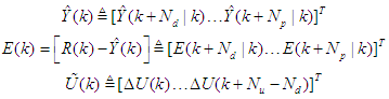
The structure of the NN-based model identification and NAMPC scheme is shown in Figure 8; where and are the desired reference signal, prediction error, control input, system output, step-delay prediction model output, step-ahead predicted output, noise/input disturbances and step-delay operator respectively and is the number of samples based on the new measurement data sample.

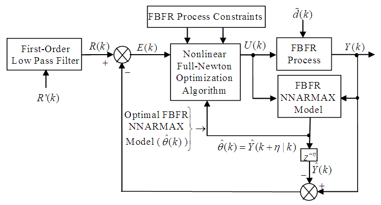Figure 8. The NN-based NAMPC scheme for the FBFR process with the NNARMAX neural network model

As in basic MPC scheme [33,34], the prediction errors E(k) between the process model and the prediction model are compensated by filtering the reference signal using a first-order low-pass digital filter defined here as:

(17)

where and are the desired reference and the filtered reference signals respectively; A_m and B_m are the denominator and numerator polynomials of the filter. In this way, the NAMPC is deigned, in part, based on the filter tracking error capability; where A_m and B_m serves as tuning parameters used to improve the robustness and internal stability of the NAMPC algorithm respectively.

The NAMPC strategy is based on a receding horizon principle illustrated in Figure 9 and depends on an explicit model of the system. The NAMPC strategy of Figure 9 is summarized as follows:

1). At the current sampling time k, the NNARMAX model predictor uses the past m-inputs, n-outputs and the current system information to identify the nonlinear discrete-time NNARMAX model of the FBFR process.

2). Assuming that at Assuming that the identified NNARMAX model is stable, proper and deterministic; then the NAMPC algorithm uses the linearized model parameters of the identified nonlinear NNARMAX model to accurately predict the current system output at that same sample time instant k.

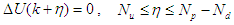
3). At time , the NAMPC algorithm calculates a sequence of control inputs consisting of the current and future inputs . The current input is held constant after control moves; where is the maximum control horizon. The input is calculated such that a set of approaches the desired reference signal in an optimal manner over a specified prediction horizon where and are the minimum and maximum prediction horizons respectively.

4). The predicted values are used to calculate the control signals by minimizing an objective function of the form:

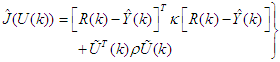(18)

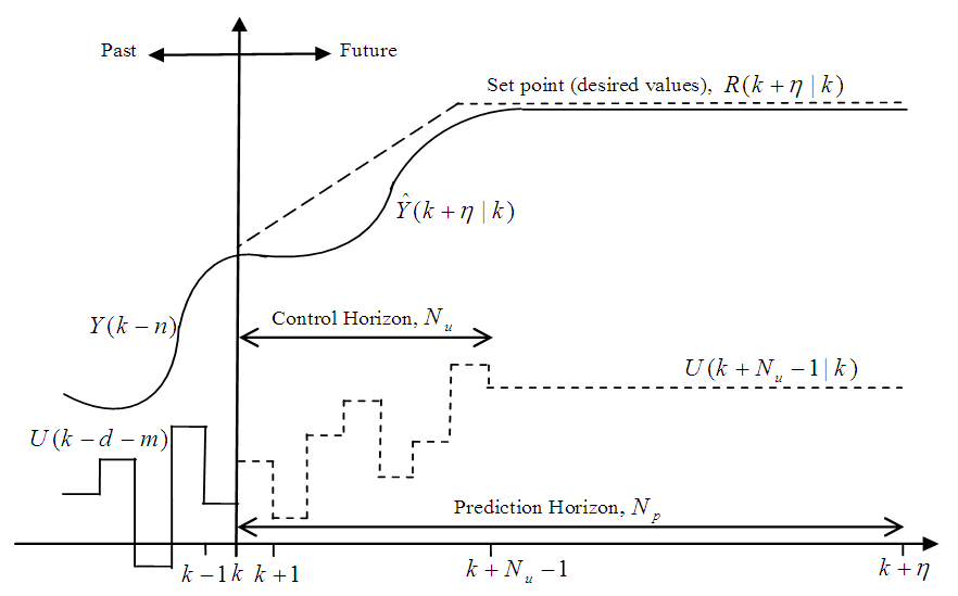Figure 9. The NAMPC strategy

subject to the constraints

(19)

(20)

where

where is the change in control signal; and are two weighting matrices penalizing changes on and in Equation (18).

Although a sequence of moves is calculated at each sampling instant, only the first control move 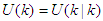is actually implemented and applied to control the process. The remaining control signals are not applied because at the next sampling instant a new output is known based on new measurements. The NAMPC strategy enters a new optimization loop while the remaining control signals are used to initialize the optimizer. This is indeed the receding horizon principle inherent in MPC strategy.

The NAMPC algorithm based on the full-Newton optimization used in this work is taken from the [33,34], where it has been demonstrated to be suitable for the control of the FBFR process [33]. Hence, the effort in this work is directed towards the online closed-loop implementation of the model identification and NAMPC schemes on the proposed NCS based on SOA technology via DPWS clients and servers to reduce the computation time at each sampling instant as well as reduced wiring and connections over long distance between the control computer and the industrial nonlinear FBFR process.

4.3. Classical PID Controller

Proportional-integral-derivative (PID) controllers are widely used in many industries because of their simple structure, robust performance and the ease of their implementation [36]. The discrete-time PID controller is defined as follows

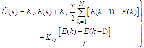(21)

where and are the proportional, integral and derivative gains respectively, is the sampling time and is the error term defined as the difference between the process and desired reference given as

(22)

The first, second and third terms in Equation (21) corresponds to the present, past and future control sequence. A major problem with PID controller is the “wind up” of the integrator resulting in saturation of the integral term for control signal of large magnitude. Rich literatures exist for anti wind-up techniques to overcome this problem [36]. According to this technique, the integrator is switched off when the actuator output exceeds a predefined limit (i.e. saturated) subject to the constraints defined in Equation (20) and updating of the integral term is stopped.

5. Neural Network-Based Model Identification and Control of the FBFR Process

5.1. Open-Loop Model Identification and Control of the FBFR Process

5.1.1. NNARMAX Model Identification of the FBFR Process

In this study, the manipulate variables for the control of the FBFR process are the high resistance potentiometer (HRP) setting which regulates the electrical energy (Q) and the flow rate of the deionized water pump (DWP) to the reactor, that is The controlled outputs of the FBFR are the temperatures of the six sections of the FBFR namely: reactor’s interior , interior reactor wall , air gap between the reactor and the heater , heater , insulator , and outer reactor metal wall ; and is expressed as

In the work carried out in [35], a well-tuned PID and MPC controllers were developed to operate the FBFR process in the range of 3.76 and 3.66 kW respectively out of the total 5.04 kW heat energy available for the process and a sampling time (T) of 2 minutes was considered for 22 hours operating cycles.

This means that 1320 data samples can be obtained from the process in one minute. In order to develop a neural network to accurately model the FBFR process in the present study, the heat supplied (Q = 5.04 kW) is varied by + 20% in order to cover the entire operating range of the pilot plant, during both initial heat-up and deactivation, and to account for the possible uncertainties in the plant model outside the operating region.

Thus, the ± 20% lower and upper values of Q are 3.528 kW and 6.552 kW respectively. Using these values of Q, the complete validated mathematical model of the FBFR process is simulated in open-loop with a sampling step of 1 minute to obtain 1320 input-output data pairs for the NN training while 300 input-output validation data is obtained from the FBFR pilot plant under normal operating condition.

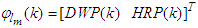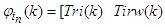
The input vector to the NNARMAX consist of the current state input regression vector and the regression vector of the six output state derivatives . The desired outputs of the NNARMAX model are the predicted values of Th and Tri given as 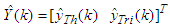. In this case, the change in the values of Q affects the FBFR outputs and can be viewed as external disturbances (see Figure 1).

The training data is scaled to zero mean and unit variance using their mean values and standard deviations according to the following equations:

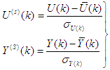(23)

where and are the mean and standard deviation of the input and output training data pair; and and are the scaled inputs and outputs respectively.

The scaling based on Equation (23) is to prevent signals of large magnitudes from dominating the identified model [34]. The network is trained for 20 epochs with the following parameters selected as: j=6, l=2, i=2, m=2, n=2 and . The four design parameters for the ARLS algorithm are selected to be: α=0.8, β=1.2, and π=0.98 resulting in γ=0.0204 which gives initial values for and equal to 0.8384 and 1.0788 respectively.

After the network training, the joint weights are rescaled afterwards according to the following expression

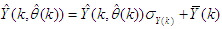(24)

so that the trained network can work with unscaled validation data collected directly from the FBFR pilot plant. The trained network is validated with 300 data obtained from the real FBFR process. The convergence of the ARLS algorithm for the real FBFR process training is shown in Figure 10. The fast convergence of the algorithm indicates its suitability for online nonlinear NNARMAX model identification of the FBFR process.

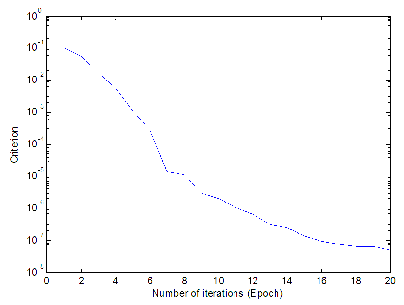Figure 10. Convergence of the ARLS training algorithm for 20 iterations for the FBFR process

The trained network is used for K-step ahead predictions [34]. The results of the K-step ahead output predictions (red --*) using the K-step ahead predictor validation method for 5-step ahead output predictions (that is, K=5) compared with the unscaled training data (blue -) are shown in Figure 11(a) and (b) for Th and Tri respectively. It can be seen that the predicted values closely track the unscaled training data.

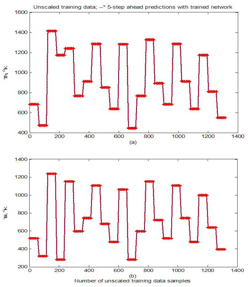Figure 11. Comparison of 5-step ahead output predictions by the trained network (red --*) with the original unscaled training data (blue -) for (a) and (b)

The computation of the mean value of the prediction error (MVPE) gives 5.6946e-004 and 6.8184e-004 for Th and Tri respectively. The small MVPE values are indications that the identified NNARMAX model approximated the dynamics of the FBFR process to a high degree of accuracy and also demonstrates the efficiency of the ARLS algorithm suitability for online NN training for use in nonlinear MPC applications as in the demonstrated in this study.

5.1.2. Temperature Control of the FBFR Process

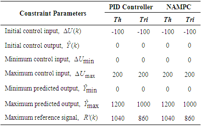
The FBFR is characterized by very high temperature at initial heat-up [34,35]. The main control objective here is to ensure that there is no overshoot in temperatures of the electric heater (Th) and the reactor interior (Tri) throughout the catalyst processing and deactivation process as a relatively small overshoot above 2% might give final product properties that would not be acceptable [35].

The desired reference signal used for evaluating the performance NAMPC and the PID controllers for the FBFR process control is based on a first-order change in temperature set-point variations similar to the one used in the original FBFR problem [34,35]. One advantage of this first-order change is to avoid aggressive response in the manipulated variables arising from a step change in the controlled variables set points. The set points calculation for the desired reference defined [34,35] is:

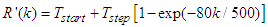(25)

where T_start and T_step denotes the temperature level before the initiation of the experiment and the step change in the temperature. Note that the coefficients in the exponential term influence the first-order response of the set point. T_start for the heater (Th) and reactor interior (Tri) are both 0°K whereas T_step for Th and Tri are 1040°K and 860°K respectively.

Initially, the NNARMAX model of the FBFR is identified and validated as in the previous sub-section to obtain the optimal network parameters. The controllers are then simulated subject to the constraints in Equation (20) defined in Table 3 and tuned using the NNARMAX model . The optimal tuning parameters obtained for the PID are and NAMPC controllers are given in Table 4. Next, the FBFR NNARMAX model is used to simulate the PID and NAMPC controllers in open-loop.

Table 3. FBFR Process Constraints

Table 4. Tuning Parameters

The open-loop PID and the NAMPC control performance for the Th and Tri output predictions are shown in Figure 12(a)–(b) while the control inputs, DWP and HRP are shown in Figure 12(c)–(d). The prediction errors due to the PID and NAMPC controllers are shown in Figure 12(e) and (f). In this simulation, we allow the constraints on the maximum predicted outputs to be 1200°K and 1000°K for Th and Tri respectively (see Table 3) in order to observe any overshoot. As it can be seen in Figure 12, the NAMPC shows good control performance over the PID controller. The PID controller exhibits overshoot with oscillations and hardly track the desired reference signals as in Figure 12(a) and (b) as well as significant output prediction errors which is evident in Figure 12(e) and (f).

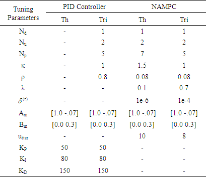
Figure 12. FBFR temperature predictions by the PID controller (blue--) and NAMPC (red) for (a) Th and (b) Tri with the control signals (c) HRP and (d) DWP for tracking the reference signal (green -.-) together with output prediction errors in (e) and (f) for Th and Tri respectively due to both controllers for k = 350 samples

5.2. Online Closed-Loop Implementation of the Model Identification and NAMPC Control of the FBFR Process Using the Proposed NCS Based on SOA Technology with DPWS

In order to evaluate the online performance of the proposed identification and control strategies, the FBFR process was considered using the proposed NAMPC due to its superior control performance over the PID controller as shown in the previous sub-section based on the architecture shown in Figure 8. The NN-based NAMPC scheme of Figure 8 is used with the NNARMAX model identification scheme of Figure 6 in closed-loop with the process (that is, the FBFR process). The complete block diagram for the online closed-loop implementation of the NNARMAX model identification and adaptive control of the FBFR using the proposed NCS based on SOA computer network via DPWS clients and servers is illustrated in Figure 13.

Figure 13. Online closed-loop implementation of the NNARMAX model identification and adaptive control of the FBFR using the proposed NCS based on SOA computer network via DPWS clients and servers

At each sampling time instant k, two new input-output data pair is obtained from the FBFR process over 120 samples of Q in steps of 60.5 Watt from 0 to 6.048 kW. The new data is progressively added to in a first-in first-out fashion as discussed in sub-section 4.1 and they also constitute the and data that are the inputs to the NNARMAX identification scheme of Figure 7. Since has been selected in sub-section 5.1.1, thus the NNARMAX model input vector consists of the current input and output states of the FBFR process at each time sample.

The current inputs as well as the new outputs produced by the FBFR process due to changes in Q are delivered to the proposed identification and control scheme over six networks: a DPWS-based Ethernet network (first network), a DPWS-based Ethernet network which uses the EXI format (second network), a DPWS-based Ethernet network which uses the IASFT format (third network), a DPWS-based switched Ethernet network (fourth network), a DPWS-based switched Ethernet network which uses the EXI format (fifth network) and a DPWS-based switched Ethernet network which uses the IASFT format (sixth network). The first three networks reside in the Ethernet networks while the last three reside in the switched Ethernet networks used in this study. The sixth network constitutes the proposed computer network. All of them consist of six sensors corresponding to six state output derivatives, two actuators for the current FBFR process inputs and one component associated with the proposed identification and control scheme. When Ethernet network is used the aforementioned components are interconnected with each other through an Ethernet bus while when the switched Ethernet is used three Ethernet switches are utilized for interconnections complying by this way with the architecture depicted in Figure 1. The performance of all networks is studied during eventing and control level interactions due to the reasons explained in Section 2.

In all networks the sensors and actuators are DPWS servers and transmit data to the proposed identification and control scheme by using the eventing level interaction while the control system is a DPWS client and communicates with the actuators by utilizing the control level interaction. All the aforementioned transactions are accomplished at each sample time. During these interactions HTTP is used and so TCP connections are established. Therefore Equation (7) can be used for calculating the worst case overall control loop delay when the switched Ethernet is used. The same equation can be used for determining the worst case overall control loop delay when the Ethernet network is used, as long as and are the overall processing delays that TCP data segments experience in the Ethernet network.

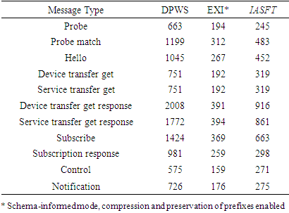
A simulation study has been made using the network simulator (NS)–2 version 2.34 [37] for determining the and in Equation (7). NS-2 supports transmissions and receptions of packets on different wires and nodes regenerate the information and only forwards it to the port on which the destination is attached. So the switched Ethernet architecture is supported. Furthermore NS-2 implements IEEE 802.3 specification and therefore the Ethernet network can be used. The adoption of the simulator is based on the fact that the worst case transmission delay requires the simultaneous transmission of data as discussed in Section 2. As soon as the simulator provides better synchronization between nodes, more accurate results could be obtained than from a real network. The simulation was made for 120 sampling periods by using half and full duplex links as a medium for connecting the components in Ethernet networks and in the switched Ethernet networks respectively. The link capacity was set to 10Mbps, and the propagation delay to 0.1 μs. In the simulator, the node that corresponds to the proposed identification and control algorithms was programmed to transmit data to the actuators as soon as it receives the current state input vector and the vector of the six output state derivatives. Moreover, a constant bit rate (CBR) application was developed that produces the eventing and control messages with 1 minute rate. This application has been developed over TCP/IP technology. Lastly, in all networks ten more nodes were used as traffic generators. These generators transmit 256 bytes of data every 1 ms in order to add additional traffic.

In Table 5 are listed the data volume of the exchanged messages that were produced from the FBFR control application from the different formats. Next a comparison is made between the six networks in order to verify the efficacy of the proposed NCS based on SOA computer network.

Table 5. Size volume of the DPWS, EXI and IASFT messages (in bytes) from the FBFR application

5.2.1. Worst Case Overall Control Loop Delay Introduced by the Ethernet Networks

In the first network the DPWS format is used while in the second the EXI format is utilized. In the third the IASFT is applied to every exchanged message.

In the first network the size of the TCP data segment transmitted from the device level to the control system is set to 972 octets. This is due to the fact that the notification message is 726 octets and is augmented with 180 octets of HTTP headers plus 20 octets of TCP headers plus 20 octets of IP headers plus 26 octets of MAC/DLL/PHY headers. Moreover, in the first network the size of the TCP data segment transmitted from the control system to the device level is set to 821 octets as the control message is 575 octets and is augmented with 180 octets of HTTP headers plus 20 octets of TCP headers plus 20 octets of IP headers plus 26 octets of MAC/DLL/PHY headers. Following the same way, in the second network the size of the TCP data segment transmitted from the device level to the control system is set to 422 octets while the size of the TCP data segment transmitted from the control system to the device level is set to 405 octets. Finally in the third network the size of the TCP data segment transmitted from the device level to the control system is set to 521 octets while the size of the TCP data segment transmitted from the control system to the device level is set to 517 octets.

The simulation results obtained are shown in Figure 14. As it is shown, in all of the three cases the network never reached a stable state and so no predictions could be made about the transmission delay due to the non-deterministic characteristic of the Ethernet network. As it can also be seen in Figure 14, in the first network the transmission delay some times exceeds the sampling period of the FBFR process.

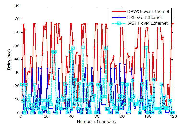Figure 14. delay between the FBFR process and the control system obtained by NS-2 when the Ethernet networks are used

In the first network, the maximum is observed to be 77.21 seconds. 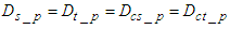which is the DPWS protocol stack response time and is defined to be approximately 10 ms [37]. Also 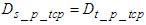and is observed to be approximately 300 μs while the average is approximately 2.7 seconds as evident in Figure 15. All the aforementioned delays were computed using an Intel® Core™ 2 CPU running at 2.66GHz. Therefore, the worst case overall control loop delay in the first network is calculated using Equation (7) to be equal with 79.95 seconds. So the DPWS-based Ethernet network cannot fulfill the real time characteristics of the FBFR process as evident in the online step response simulation result of Figure 16. The poor performance of the NAMPC in tracking the desired reference is due to the transmission delay introduced by the network. As depicted most especially in Figure 16(a), the NAMPC sometimes tracks and sometimes does not track the desired reference according to the transmission delay introduced by the network which is sometimes below or above the sampling time of the FBFR process (see Figure 14).

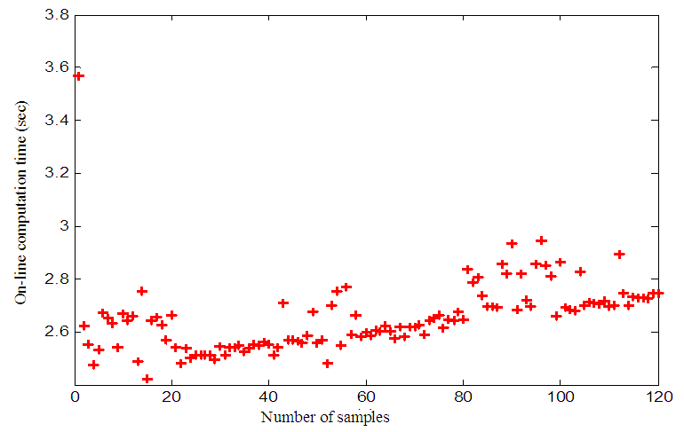Figure 15. Computation time for the online FBFR model identification and control at each time sample

Figure 16. Online identification and control of the FBFR process implemented over the first network: (a) Th and (b) Tri predictions with their respective control signals (c) HRP and (d) DWP

In the second network, the maximum is observed to be 37 seconds. Here is the DPWS protocol stack response time plus the execution time for encoding the DPWS notification message to the EXI notification message. This delay was observed to be 22 ms. Moreover is the DPWS protocol stack response time plus the execution time for decoding the EXI notification message to the DPWS notification message. This delay was observed to be 18 ms. is the DPWS protocol stack response time plus the execution time for encoding the DPWS control message to the EXI control message and is 13 ms while is the DPWS protocol stack response time plus the execution time for decoding the EXI control message to the DPWS control message and is 22 ms. and seconds. All the aforementioned delays were computed using an Intel® Core™ 2 CPU running at 2.66GHz. Therefore, the worst case overall control loop delay in the second network is calculated using Equation (7) to be equal with 39.81 seconds.

In the third network, the maximum is observed to be 48.9 seconds. Here is the DPWS protocol stack response time plus the execution time of the XSLT processor for producing the IASFT notification message from the DPWS notification message. This delay was observed to be 13 ms while in Figure 2 it has been shown how the IASFT mechanism transforms the DPWS notification message from the FBFR application to the equivalent IASFT notification message. Moreover is the DPWS protocol stack response time plus of the XSLT processor for producing the DPWS notification message from the IASFT notification message. This delay was observed to be 5 ms. is the DPWS protocol stack response time plus the execution time of the XSLT processor for producing the IASFT control message from the DPWS control message and is 14 ms while is the DPWS protocol stack response time plus the execution time of the XSLT processor for producing the DPWS control message from the IASFT control message and is 5 ms. and = 2.7 seconds. All the aforementioned delays were computed using an Intel® Core™ 2 CPU running at 2.66GHz. Therefore, the worst case overall control loop delay in the third network is calculated using Equation (7) to be equal with 51.67 seconds.

In the second and third network the worst case overall control loop delay is below the sampling period of the FBFR process. Therefore these two networks fulfill the real time requirement of the FBFR process as shown in the online step response simulation result of Figure 17 where the NAMPC tracks the desired reference signal at each sampling instant. When the EXI format is used the DPWS-based Ethernet network introduces the minimum worst case overall control loop delay between the Ethernet networks. However the interoperability feature is lost as binary-based encoding is utilized. On the other hand, the IASFT renders the DPWS-based Ethernet network suitable for controlling the FBFR process while XML and DPWS standards are not distorted.

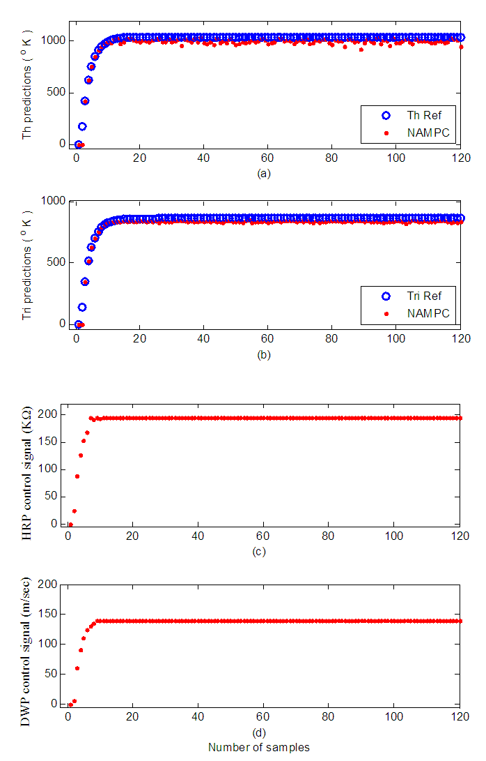
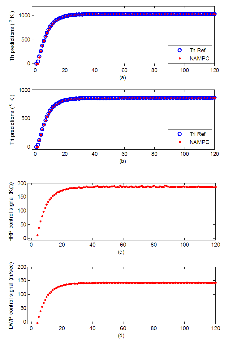Figure 17. Online identification and control of the FBFR process when the worst case overall control loop delay introduced by the utilized network is below the sampling period of the FBFR process: (a) Th and (b)Tri predictions with their respective control signals (c) HRP and (d) DWP

5.2.2. Worst Case Overall Control Loop Delay Introduced by the Switched Ethernet Networks

In the fourth network the DPWS format is used while in the fifth the EXI format is utilized. In the sixth network the IASFT is applied to the exchanged messages.

In the fourth, fifth and sixth networks all the delays except from the as well as the data volumes of the exchanged messages are the same with the ones computed for the first, second and third networks respectively.

The simulation results obtained using the NS-2 are shown in Figure 18. In the fourth, fifth and sixth network the was observed to be 0.023 seconds, 0.012 seconds and 0.014 seconds respectively at each sampling time (except from the first one). Therefore the worst case overall control loop delays for the fourth, fifth and sixth networks are calculated using Equation (7) to be equal with 2.77, 2.82 and 2.78 seconds respectively.

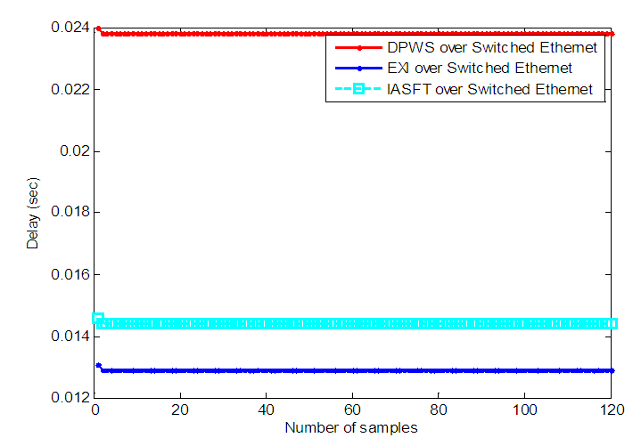Figure 18. delay between the FBFR process and the control system obtained by NS-2 when the switched Ethernet networks are used

The round trip delays between the DPWS clients and sensors are shown in Figure 19. It is obvious that the worst case overall control loop delays have been significantly reduced when compared with the delays introduced by the Ethernet networks due to the switched Ethernet architecture.

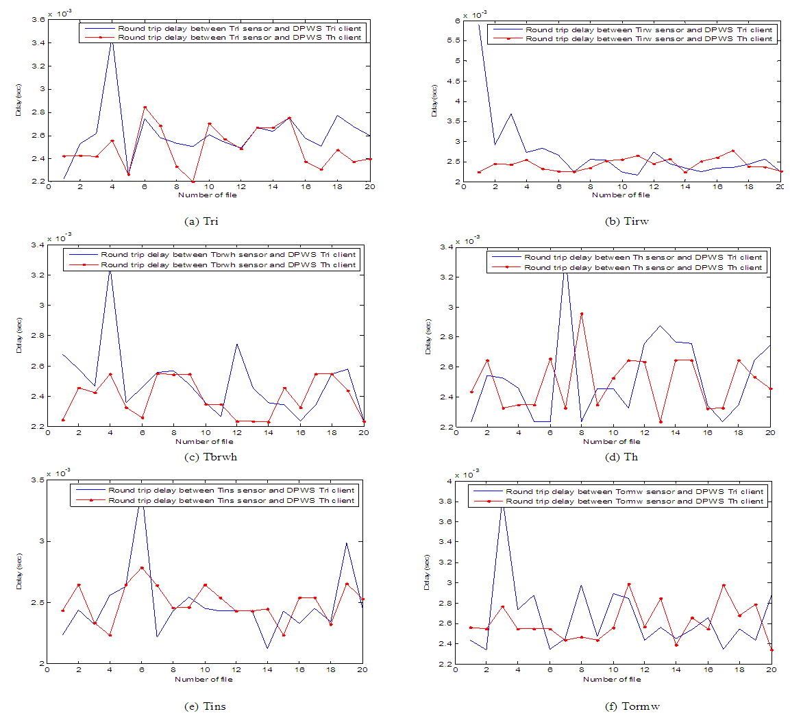Figure 19. Round trip delays between DPWS clients (on Tri and Th controllers) and sensors (a) Tri, (b) Tirw, (c) Tbrwh, (d) Th, (e) Tins and (f) Tormw

In all networks that use the switched Ethernet architecture the worst case overall control loop delay is below the sampling period of the FBFR process. Therefore the real time requirement of the FBFR process is fulfilled as shown in the online step response simulation result of Figure 17. When the EXI format is used the DPWS-based switched Ethernet network introduces the minimum transmission delay between the last three networks. However the interoperability feature is lost. Moreover the worst case overall control loop delay is the maximum because of the execution time needed for encoding and decoding the EXI messages. On the other hand, not only does not the IASFT mechanism distort the XML and DPWS standards but it also transforms the DPWS to IASFT messages and vice versa with less execution time as it is based on XSLT stylesheets.

6. Conclusions

The superior control performance of the NAMPC combined with the NNARMAX model trained using the ARLS algorithm for the FBFR online model identification and control demonstrates the suitability of the NCS over a SOA computer network based on the device profile for web services (DPWS). The worst case overall control loop turnaround time was 12.8465 seconds. Results obtained shows that the implementation of the online NNARMAX model identification and the NAMPC algorithms using NCS over the SOA computer network based on DPWS meets by far the limit imposed by the upper limit of the FBFR sampling time and therefore they can be deployed for the FBFR process control in an industrial environment. Furthermore the new SOA computer network offers interoperability between its components by using a DPWS technology combined with a new compression technique as well as a bounded worst case overall control loop delay.

Developments and implementations of NCSs for industrial control applications are still in progress. The conventional components in NCS include sensors, actuators, industrial plant (or process) controller as well as the communication network topologies, nodes and devices. The main difference between conventional control and NCS lies on the mode of communication that connects the sensors, actuators, industrial plant (or process) and the controller. The main challenge in NCS is transmission delay introduced by the communication networks.

In this work, however, simulation results have shown that the new compression technique is able to render even the DPWS-based traditional Ethernet network suitable for the online control of the FBFR process. Furthermore, the obtained transmission delay is significantly reduced when the proposed computer network is used. Despite the transmission delay introduced by the proposed computer network, no overshoot was observed during the online implementation of the proposed NAMPC. By this way the control objective is satisfied. The aforementioned characteristics render the proposed computer network suitable for industrial control applications.

ACKNOWLEDEGMENTS

The authors wish to thank Dr. S. S. Voutetakis of the Hellenic Center for Research and Technology, Thermi – Thessaloniki, Greece for providing all the information required to model the SDU and the FBFR as well as data from the operation of this unit.

Conflict of Interest

The authors declare that they have no conflict of interest.