-
Paper Information
- Paper Submission
-
Journal Information
- About This Journal
- Editorial Board
- Current Issue
- Archive
- Author Guidelines
- Contact Us
International Journal of Control Science and Engineering
p-ISSN: 2168-4952 e-ISSN: 2168-4960
2021; 11(1): 1-8
doi:10.5923/j.control.20211101.01
Received: Aug. 9, 2021; Accepted: Aug. 25, 2021; Published: Sep. 15, 2021

Stochastic Dynamic Systems’ State Estimation Based on Mean Squared Error Minimizing and Kalman Filtering
 Abstract
 Reference
 Full-Text PDF
 Full-text HTML
Bukhar Kussainov
Institute of Heat Power Engineering and Control Systems, Almaty University of Power Engineering and Telecommunications, Almaty, Republic of Kazakhstan
Correspondence to: Bukhar Kussainov, Institute of Heat Power Engineering and Control Systems, Almaty University of Power Engineering and Telecommunications, Almaty, Republic of Kazakhstan.
| Email: |  |
Copyright © 2021 The Author(s). Published by Scientific & Academic Publishing.
This work is licensed under the Creative Commons Attribution International License (CC BY).
http://creativecommons.org/licenses/by/4.0/

In automatic control systems, telecommunications and information systems subjected to impact of random disturbances and measurement inaccuracies, there is the problem of estimating the state vector of observed stochastic system. With the aim to solve the problem the state space system model is described and the problem statement is given. To solve the problem it’s used the discrete Kalman filter (KF) presenting itself the recurrent procedure in the form of the set of the difference vector-matrix equations. In the paper the way of deriving the equations of KF on the basis of the procedure of minimization of the mean-squared error of estimation based on a method of the least squares is considered. Using this procedure the discrete analog of the Wiener-Hopf equation as well as Gaussian and Gaussian-Markov estimates of the state vector of linear stochastic system are received satisfying to a minimum of the mean-squared error in the estimate. On the basis of the received estimates and the discrete equation of Wiener-Hopf the equations of the KF is derived, the theorem of the KF with the minimum mean-squared error is formulated, the sequence of using the equations of KF making up the recursive algorithm of KF for computer program realization is explained.
Keywords: Stochastic systems, State estimation, Kalman filter
Cite this paper: Bukhar Kussainov, Stochastic Dynamic Systems’ State Estimation Based on Mean Squared Error Minimizing and Kalman Filtering, International Journal of Control Science and Engineering, Vol. 11 No. 1, 2021, pp. 1-8. doi: 10.5923/j.control.20211101.01.
Article Outline
1. Introduction
- Modern automatic control systems as well as telecommunications and information systems transmitting and processing signals and subjected to impact of random perturbations and uncertainties of system parameters and to influence of random external disturbances and measurement noises can be considered in the form of the state space models of non-stationary linear dynamical stochastic systems [1]. In stochastic systems, to realize modern control algorithms or to separate a useful signal from its mixture with noise, there is a problem of estimating the entire state vector of the dynamical system based on measured values of system’s output signal [2]. The solution of this problem in real time is a filtering problem, for which the classical and most popular solution algorithm is the discrete Kalman filter (KF) [3,4], using both in control theory and in the theory of signal transmission and processing [5]. The KF has the same structure as the considered dynamical system, is the mathematical model and consists of a set of difference vector-matrix equations for calculating estimates of the state of a stochastic system, estimates of the error covariance matrices and the filter gain. The difference between it and the system is that at any given time, the filter gain is optimal relative to the specified statistical properties of disturbances and measurement errors [2-8]. The computational algorithm of the KF is a recursive procedure that is convenient for program realization using programming languages as well as MATLAB [3,9-11] and other computer programs for system modeling.The article presents a mathematical model of a discrete non-stationary linear stochastic dynamical system, the formulation of the problem of estimating the vector of the system state, the derivation of equations and the formulation of the KF theorem, as well as an algorithm for using the equations of the discrete KF. As it’s known, the estimation of the state of a dynamical system (the solution of the filtration problem), as well as the derivation of the KF equations can be carried out using the Bayesian approach, maximum likelihood estimation or the least squares method [12]. Here we follow the already known path and consider the filtration problem as a generalization of the Gaussian least squares method, described in detail in [13]. Based on the least squares method and the procedure for minimizing the mean-squared error of estimation, a discrete analog of the Wiener-Hopf equation is obtained, as well as Gaussian and Gaussian-Markov estimates (and estimates of their error covariance matrices) of the state vector of the observed system, which are linear unbiased and satisfy the minimum value of the mean-squared error of estimation [13]. The discrete Wiener-Hopf equation, Gaussian and Gaussian-Markov estimates with a minimum mean-squared error are used later to derive the discrete KF equations, that are a recurrent procedure in which at a discrete time
 of the extrapolation (prediction) stage, based on the difference equations of the dynamics of the observed system, the estimate of the state vector is calculated for the next
  moment of time, and then, at the time
  of the correction stage, based on new measurement of the system output signal and the changed value of the KF gain, the estimate of the state vector of the system calculated at the time
  of extrapolation of the KF procedure is corrected [2-13].From the first application of the KF in the airspace the KF was a part of the Apollo onboard guidance [3] and to our days the KF has been demonstrating its usefulness in many various applications in different areas of technology and economics [14-16]. However, it is still not easy for people who are not familiar with the estimation theory to understand and implement the vector-matrix equations of the KF. Whereas there is a large number of excellent introductory materials and literature on the KF the purpose of this paper is to remind one simple method for deriving and explain the recursive algorithm for using the equations of the KF.
 2. Notational Preliminaries
- All vectors and matrices are time-varying quantities are treated at the discrete time instants
 . By convention, the argument
  of vectors (e.g.,
  …) and matrices (e.g.,
  …) denotes the fact that the values of these variables correspond to the
  th step of time. The notation
  designates that the value of the estimation vector
  at the time instant
  conditioned on
  time instant measurements. If
  we are estimating a future value of
  , and we refer to this as a predicted estimate. The case
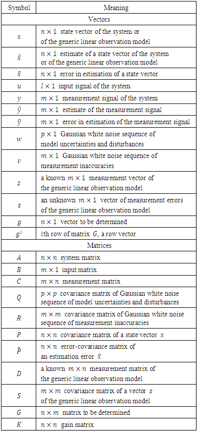
  is referred to as a filtered estimate. Prediction and filtering make up the algorithm of KF and can be done in real time [6-8].The list of notations used through the paper is summarized in the Table 1.
|
3. The Basic Model and the Problem of the State Estimation
- Consider the basic linear, time-varying (nonstationary), discrete-time state variable model of dynamical systems [5,6] as:
 | (1) |
 | (2) |
 is a
is a  state vector;
  is a
is a  measurement vector;
  is
is  input vector;
  is
is  system matrix;
  is
is  input matrix;
  is
is  measurement matrix.
  ,
,  ,
,  matrices and
  vector are known.Additionally,
  is
is  Gaussian white noise sequence of model uncertainties and disturbances and
  is
is  Gaussian white noise sequence of measurement inaccuracies, i.e.,
 | (3) |
 | (4) |
 denotes the matrix transposition.
 ,
,  are
are  and
and  covariance matrices, respectively,
  is the Dirac delta function, i.e.,
  for
for  and
and  for
for  . Supposed that
  and
and  are mutually uncorrelated, i.e.,
 | (5) |
 is zero mean and has a
  covariance matrix
  , i.e.,
 | (6) |
 and its covariance matrix
  are known and
  is uncorrelated with
  and
and  , i.e.,
 | (7) |
 unknown state vector
  at
at  from the
  noisy measurement vector
  , where
  .The estimate
  of a state vector
  must be: 1) linear, 2) unbiased, i.e.,
  and must have 3) a minimum value of the mean of the squared error
  , i.e.,
 | (8) |
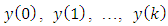
 is the error in the estimate.Thus, there is the mean-squared estimation problem: given the noisy measurements
  determine a linear unbiased estimator of the entire state vector
  such that the conditional mean-squared error in the estimate
 | (9) |
 can also be called as the minimum variance estimator, since
  | (10) |
 variances are diagonal elements of
  error-covariance matrix defined by [6]:
 | (11) |
4. The Method of Minimizing of the Mean-Squared Error of Estimation
- To obtain the expressions for estimates
 of unknown vector
  from the measurement vector
  in conditions of measurement noises
  according to the Eq. (2) let’s consider the generic linear observation model [5]:
 | (12) |
 is an
is an  unknown vector,
  is a known
  measurement vector,
  is a known
  measurement matrix,
  is an unknown
  vector of measurement errors.The unknown quantities
  and
and  are random variables with the following expectations and covariance matrices and they are mutually uncorrelated, i.e.:
 | (13) |

 | (14) |
 vector
  and
and  matrix
  must determine, however, the request of the unbiased estimation means that:
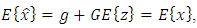 hence
hence  since
since 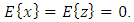 Thus the Eq. (14) for
  becomes as:
 | (15) |
 will be determined from the condition that the variance of estimation error
  is minimum. According to Eq. (15) every component
  of
of  is depended on vector
  via an
  row of matrix
  which is denoted as
  Thus
Thus | (16) |
 is the row vector.Mentioned request about a minimum variance of estimation error signifies that
 | (17) |
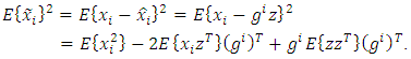 | (18) |
 error is the sum in which the first term don’t depend on
  , the second and third terms are linear and quadratic forms of
  is the column vector). A necessary condition of minimum of Eq. (18) is that all its partial derivatives with respect to
  must be equal to zero. In other words, taking the gradient of
  with respect to
  must be equal to zero, i.e.,
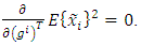 | (19) |
 | (20) |
 | (21) |
 is that the variance
  of each
  estimation error must be extremum. The sufficient condition of it is the positive definiteness of the matrix formed by the second derivatives of the function
  with respect to
  . In other words, the Hessian matrix with respect to
  must be positive definite for all
  i.e.:
i.e.: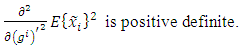 | (22) |
 | (23) |
 .To obtain the matrix
  we must find the covariance matrices in Eq. (21), so taking into account the Eqs. (12), (13) we have:
 | (24) |
 | (25) |
 | (26) |
 matrix. If
  measurements are less than
  unknowns, then from the Eq. (26) we can find the matrix
  :
: | (27) |
 | (28) |
 | (29) |
 | (30) |
 | (31) |
 | (32) |
 measurements are more than
  unknowns, the Eq. (26) can be transformed to the following form [13]:
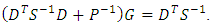 | (33) |
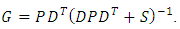
 matrix. Using matrix
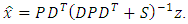
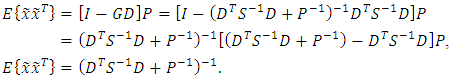
  obtained from the Eq. (33) the second form of the linear unbiased estimate with a minimum value of mean-squared estimation error is:
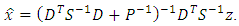 | (34) |
 | (35) |
 that is
  and rank of matrix
  is
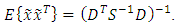
is  then we have the Gaussian-Markov estimate [13]:
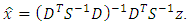 | (36) |
 | (37) |
5. Deriving the Equations of the Kalman Filter
- The Kalman filter operates in a predict-correct manner [5].
5.1. Prediction
- At the initial observation moment according to the Eqs. (2), (6) the following measuring is obtained:
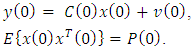 | (38) |
 | (39) |
 | (40) |
 | (41) |
 to
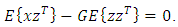
to  With this aim consider the discrete Wiener-Hopf equation (21) which is the necessary and sufficient condition that estimate will have a minimum mean-squared error. Rewrite Eq. (21) in more short form:
 | (42) |
 are already done and the estimate
  with the minimum of the mean-squared error is obtained. The latter means that the Eq. (42) is satisfied, i.e.:
 | (43) |
 and
and  at the time
  and
and  are known. According to the Eq. (1) let’s find the predicted value of
  herewith uncertainties and disturbances
  (with zero expectations) are not taken into account:
 | (I) |
 is optimal. According to Eq. (42) we have:
 | (44) |
 with
with  from the Eq. (1), herewith disturbances
  cannot be taken into account because they are not correlated with
  We have the following equation:
 | (45) |
 | (46) |
 however, the noises
  are not correlated with the estimation errors
  , so
, so | (II) |
5.2. Correction
- The estimate of the predicted state vector
 at the
  instant of time,
  , obtained with the available
  measurement (Eq. (I)), after the next
  measurement must be corrected to the value
  In order to find
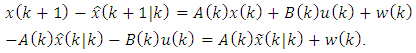
  let’s replace
  in Eq. (I) with
  and substitute instead of
  the corresponding expression from the Eq. (1):
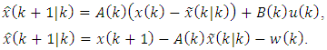 | (47) |
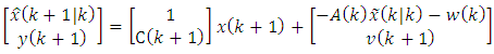 | (48) |
 | (49) |
 are defined through comparing the Eqs. (48), (49). The covariance matrix of the upper part of vector
  was earlier denoted as
  , the covariance matrix of the lower part
  is equal to
  . Covariance between
  and
and  and between
  and
and  are equal to zero. So, we have:
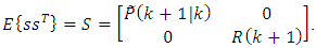 | (50) |
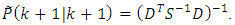
 contains the component
  we can calculate Gaussian-Markov estimate
  at the
  instant of time according to the Eqs. (36), (37), i.e.:
 | (51) |
 | (52) |
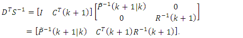 | (53) |
 | (54) |
 | (55) |
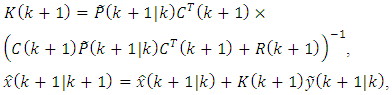
 from the Eq. (55) into the Eq. (51) of Gaussian-Markov estimate:
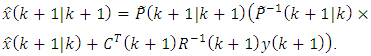 | (56) |
 is the gain matrix
  :
: | (57) |
 and taking into account the Eq. (52) we receive:
  | (58) |
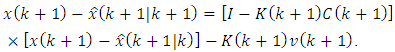
 on the left the Eq. (58) and taking into account the Eq. (57) we receive:
 | (59) |
 from the Eq. (59) and substitute it into the Eq. (56):
 | (III) |
 on the right the Eq. (59):
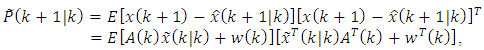
 and from this equation we can receive the error-covariance matrix:
 | (IV) |
 on the right and ascribe to the first tirm in the right hand side the factor
  From the obtained equation taking into account the Eq. (57) we can find the gain matrix
  :
: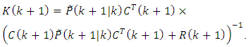 | (V) |
6. The Theorem of the Kalman Filter
- The Eqs. (39)-(41) and (I)-(V) make up together the Kalman filter which is usually formulated as the theorem. Let’s present the formulation of the theorem of Kalman filter satisfying the minimum of mean-squared error of estimation.Theorem (The Kalman Filter). Let given a discrete stochastic system defined by the Eqs. (1)-(7) and considered at
 instants of time. The linear unbiased estimate with the minimum mean-squared error in the estimation of the state vector of this system at any time instant
  is obtained by the recursive equations (I)-(V) the initial state of which at
  is determined by the equations (39)-(41).In addition to the proof of the theorem considered above to check the correctness of the Eqs. (IV), (V). With this aim let’s make the expression for
  according to the Eq. (42):
 | (60) |
 | (61) |
 and calculate expectation. Still, using the Eq. (42) will allow us to obtain the Eq. (IV).To check the correctness of the deriving the Eq. (V), consider the first part of the mathematical expectation in Eq. (60), containing values from
  to
to  and located to the left of the vertical line for
  . The new measurement error
  is uncorrelated with the old observations from
  to
to  . The product of two expressions in square brackets in (61), correlated with the set of observations from
  to
to  , means zero mathematical expectation according to equation (44). This means that expression (III) satisfies the part of the requirement (42) that is to the left of the vertical line. The remaining part of the requirement (60) allows us to determine the undefined gain matrix
  . On the basis of (61), the following equality must be valid:
 | (62) |
 and
and  are not correlated with
  . The rest of the mathematical expectations can be represented in a simpler form. To do this, we use Eq. (29) with respect to
  , taking into account that the covariance between
 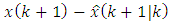 and
and  can be replaced by
  . As a result, we have:
 | (63) |
 we’ll receive the Eq. (V).
7. The Algorithm of Using the Equations of the Kalman Filter
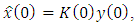
- The Kalman filter is a recursive procedure that is convenient for program realization on computers. The algorithm of using the Eqs. (39)-(41) and (I)-(V) of KF is the following as:1) At the initial state
 the initial estimate of the state vector
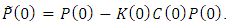
  and the initial error-covariance matrix
  are built according to the Eqs. (39)-(41):
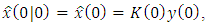 where
where  and
and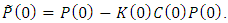 2) The estimate and its error-covariance matrix are extrapolated to the next
  observation instant of time according to the Eqs. (I), (II):
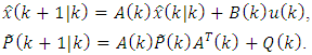 Correction:3) The optimal gain matrix
  is calculated according to the Eq. (V) and extrapolated (predicted) estimate
  is improved to the value
 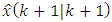 according to the Eq. (III) using the new measurement
  :
: where
where is called the innovation process,
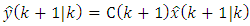 is called the predicted value of the new measurement.4) The error-covariance matrix
 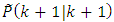 of the new modified estimate
  is calculated according to the Eq. (IV):
 5) If the next
  is
is  then the current time instant
  should be considered as
  For the estimate of the state calculated at the step 3 and now considered as
  for the error-covariance matrix calculated at the step 4 and now considered as
  should be carried out the steps 2, 3 and 4 of the algorithm. If
  then the procedure is ended.Therefore, the best estimate of
  using all observations up to and including
  is obtained by a predictor step,
  and a corrector step,
  The predictor step uses information from the state equation (1). The corrector step uses the new measurement available at
  The correction is the error (difference) between new measurement,
  , and its best predicted value,
  , multiplied by weighting (or gain) factor
  . The factor
  determines how much we will alter (change) the best estimate
  based on the new observation, i.e., 1) if the elements of
  are small, we have considerable confidence in our model, and 2) if they are large, we have considerable confidence in our observation measurements. Thus, the KF is a dynamical feedback system, its gain matrix and predicted- and filtering-error covariance matrices comprise a matrix feedback system operating within the KF [5,6].
8. Conclusions
- The discrete Kalman filter, developed by R. Kalman back in 1960 [19], is currently a classic result of the theory of control systems and the theory of signal processing, as well as the most popular filtering algorithm using in automatic control systems, telecommunications and information systems subjected to random disturbances and measurement inaccuracies. The Kalman filter is a recursive procedure consisting of difference vector-matrix equations for calculating estimates of the state of a stochastic system, the estimates of the error covariance matrices and the filter gain. A common approach to the derivation of the KF equations is the Bayesian approach [11]. The paper describes the simplest way to obtain the KF equations, based on the use of the procedure for minimizing the mean-squared error of estimation, which is a further generalization of the least squares method [12]. As a result of this procedure, we obtained: a discrete analog of the Wiener-Hopf equation, as well as Gaussian and Gaussian-Markov estimates (and their error covariance matrices), which are linear and unbiased and satisfy the minimum value of the mean-squared error of the estimation. Based on the discrete Wiener-Hopf equation, Gaussian and Gaussian-Markov estimates, the KF equations are obtained using simple algebraic transformations and reasoning. The KF theorem is formulated, which satisfies the minimum of mean-squared error of estimation, and the algorithm for using the KF equations, which is convenient for program realization, is also explained.