1. Introduction

Stability and control of nonlinear systems with control inputs is in no doubt one of the popular research interest in modern systems and control theory when compared to linear systems and has attracted lots of research [1,2,3,4] because of its wide range of applications. There are several studies on the stability [5,6,7] and controllability [8,9] of nonlinear control systems aimed at providing desired response to a design goal. The stability analysis and control synthesis of nonlinear control systems play significant role in many real life control problems which includes stabilizing, tracking, and disturbance rejection or attenuation of systems.

A nonlinear control system is considered as a system in which the static characteristics between input and output have a nonlinear relationship. A significant interconnection used for nonlinear control systems is the feedback configuration. The effect of feedback on system response depends on the design goals and several formulations of such nonlinear control problems and method of approach exists in classical control theory see for example [10,11,12] and [13]. A feedback system could be a negative or positive and is often referred to as a closed-loop system. In a feedback system, a fraction of the output values is ‘fed back’ and either added to (positive feedback) or subtracted from (negative feedback) the original set reference point. That is; the output continually updates its input in order to modify the system responses and improve stability. Several methods are used to analyze or improve the stability and stabilization of nonlinear control system which as seen in [14,15] and references therein includes fixed point based, spectral radius and the Lyapunov based.

The stability and stabilization of nonlinear control systems has been studied by many including [7,16] and [17]. For example, in [16], the stabilization of second-order systems by non-linear position feedback was investigated by placing actuators and sensors in the same location; and using a parallel compensator to obtain asymptotic stability results for the closed-loop system by LaSalle’s theorem. In [17], the stabilization of second order system with a time delay controller was analyzed using Padẽ approximation to obtain stability regions by constrained optimization; these regions are then used to optimize the impulse response of the closed loop systems and approximated the performance index with James-Nichols-Philips theorem. The spectral conditions for stability and stabilization of nonlinear co-operative systems associated to vector fields that are concave was studied in [18], using spectral radius of the Jacobian for the system where they provided conditions that guaranteed existence, uniqueness and stability of strictly positive equilibria. The fixed point and stability of nonlinear equations with variable delays was investigated in [19], were they obtained conditions for the boundedness and stability of the system using contraction mapping principle.

In [7], new stability and controllability results for nonlinear systems were established in their study of the stability and controllability of nonlinear systems using the Lyapunov and Jacobi’s linearization methods to obtain their stability results; and the rank criterion for properness for their controllability results.

The focus on this paper is the Lyapunov based approach which includes the direct and indirect method of Lyapunov. Even though the Lyapunov direct method is an effective way of investigating nonlinear systems and obtaining global results on stability of systems. This research follows similar standpoint with that of [7] by using the Lyapunov indirect method, where instead of looking for a Lyapunov function to be applied directly to the nonlinear system; the idea of linearization around a given point is used to achieve stability on some region [20] using quadratic Lyapunov functions but extends their results by designing state feedback controller for the stabilization of such systems. Next, we use the Lyapunov-Razumikhin method to explore the possibility of using the rate of change of a function on to determine sufficient condition for the stabilization of the feedback system.

The rest of the paper is organized in the following order; Section 2 contains preliminaries and definitions on the subject areas as guide to the research methodology. Section 3 contains stability results on the equilibrium point for the system while Section 4 contains the main results of this research; with application and simulation output result illustrating the effectiveness of the study given in Section 5 prior to the conclusion in Section 6.

2. Preliminaries and Definitions

Let is a real dimensional Euclidean space with norm is the space of continuous function mapping the interval into with the norm where Define the symbol Here, we consider only initial data satisfying the condition that is, for all

2.1. Preliminaries

We consider the autonomous system

(1)

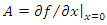
where and is a continuously differentiable function and define

(2)

where, are and constant matrices respectively, , and denotes the Jaciobian matrix. satisfies the condition

Consider system (1) with all its necessary assumptions given by

(3)

and its free system

(4)

2.2. Definitions

We now give some definitions that underpins the subject areas of this research work.

Definition 2.1. The equilibrium point of system (3) is stable if for any there exists a such that if implies for

Definition 2.2. The equilibrium point of system (3) is asymptotically stable if it is stable and there is such that implies as

Definition 2.3. The solution of system (3) is uniformly stable if Definition 1 is independent of

Definition 2.4. The solution of system (3) is uniformly asymptotically stable, if it is uniformly stable and there exist such that every there is a such that implies for .

3. Stability Result

Consider system (1) with given by

(5)

Theorem 3.1. Lyapunov’s indirect method

If is an equilibrium point for the system (5) with for all Let

(6)

be the Jacobian matrix of with respect to at the origin such that

(7)

and assume that

(8)

Furthermore, let be defined by equation (6), so that it can be approximated by (4).

Then, the origin is

a. Asymptotically stable if the origin of the linearized system (5) is asymptotically stable, i.e. if the matrix A is Hurwitz namely the eigenvalues of A lies on

b. Unstable if the origin of the linearized system (5) is unstable i.e. if one or more eigenvalues of A lie in the open right-half of the complex plane.

Proof: The proof is given in [7] and therefore omitted.

4. Feedback Control of System

The main results of this paper will be stated as theorems in this section.

The proofs of the next two theorems follow along the lines of the proofs of Theorem 4.1and 4.2 in [21].

Theorem 4.1. Suppose there are continuous non-decreasing, nonnegative functions with for and and there is a continuous function

such that

(i)

(ii) , for all satisfying . Then the zero solution of system (3) is uniformly stable.

Theorem 4.2. Let be the function satisfying condition (i) in Theorem 4.1, and if in addition there exists constant a continuous non-decreasing, nonnegative functions for and a continuous function for such that condition (ii) in Theorem 4.1 is strengthened to

(iii) 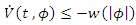for all satisfying . Then the zero solution of (3) is uniformly asymptotically stable.

4.1. Main Results

Theorem 4.3. Consider system (1), with all its assumptions. If and the linearized system

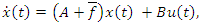(9)

where, and 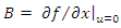is such that is a controllable pair. Then, there exists a matrix such that all the eigen-values of are in Furthermore, using the control law the equilibrium is asymptotically stable for the closed loop system.

Proof. Assume that is controllable, then by the Hautus criterion for controllability for some We proof by contraposition. Assume that for some then by the Kalman controllability decomposition lemma; there exists such that:

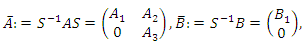where the pair 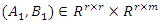is controllable with Now, the equilibrium of the linearized system (9) will be asymptotically stable if there exist such that

(10)

That is, all eigenvalues of have negative real parts. Defining we have

Let and be eigenvalue/eigenvector pair of so that setting

it follows that

Consequently, showing that and

(11)

Also, by the stability criteria and therefore

(12)

by (10) and (11). Now setting we get

Therefore, by (4.4) and the theorem is proved.

We now use the Razumikhin method to find the uniform asymptotic stability of the system. It is known from theorem of Lyapunov matrix equation that, there is a symmetric positive definite matrix such that where I is the identity matrix and is the transpose of be positive numbers such that and are the least and greatest Eigen-values of respectively. Then, it is clear that, 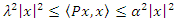, for all . Making use of the assumptions on the equation (3) we now develop a new theorem for uniform asymptotic stability.

Theorem 4.4. Let all the assumptions on system (3) be satisfied, such that is a controllable pair and suppose,

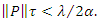(13)

Then, the exists a matrix such that using the control law the equilibrium of the closed loop system

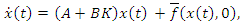(14)

is uniformly asymptotically stable.

Proof. Given relation (13), choose a constant so that 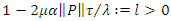. Now, let . It is necessary to prove that satisfies all the conditions in Theorem 4.2 for system (14). It is obvious that conditions (i) of Theorem 4.1 holds, assume now that 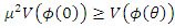, so that 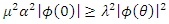and hence for all Then, the derivative along the solution of equation (14) is given by

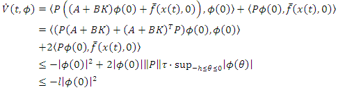Thus, the condition of Theorem 4.2 holds if and there is a such that If in addition and Then, the zero solution of system (14) is uniformly asymptotically stable.

5. Illustrative Examples

Consider the modeling of a mass spring damper with mass attached to a damper and a nonlinear spring in [7] with all its necessary assumption given by

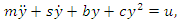(15)

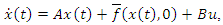which when transformed into state space takes the form where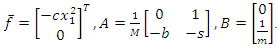

Example 5.1

If the nonlinear system (15) is estimated by

(16)

The stability of system (16) with using Theorem 3.1 when evaluated gives two points of equilibrium 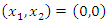and and Jacobian matrix is obtained as

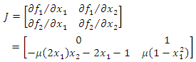Evaluating the Jacobian at these two points gives

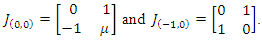The linearized system matrix at equilibrium is a stable point for for all and unstable point for with and Since is stable point for all the first assumption of Theorem 3.1 is satisfied i.e. is an equilibrium point for all Next, we show that condition (8) of Theorem 3.1 is satisfied as follows. Let

Thus, condition (8) is satisfied, hence system (16) is asymptotically stable.

We now use the control law to stabilize the system, where

Observe by Theorem 4.3 that,

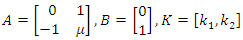so that,

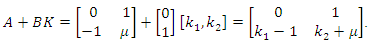Hence, for and That is and For simulation purposes with the feedback control law, we let and The simulation output with the feedback control law is given in Figure 1.

Figure 1. Open and closed-loop responses of the system

Example 5.2

Let and be defined as in Example 5.1 with

be the symmetric positive definite matrix with and as the least and greatest eigenvalues respectively. Using the control law system (16) can be written in the form of equation (14) to be of the form

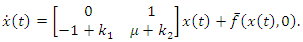(17)

Observe first that the pair is controllable and the function satisfies the condition 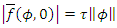with Check also that, 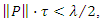which satisfies the condition of Theorem 4.4. Moreover,

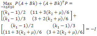and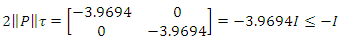

Therefore, the zero solution of system (14) is uniformly asymptotically stable.

6. Conclusions

In this paper, the stability and feedback control results of nonlinear systems are presented with examples given. The Lyapunov indirect method and the Jacobian linearization methods were used to analyze stability and the stabilization of the system using feedback control law. Furthermore, the Lyapunov-Razumikhin method was used to determine sufficient conditions for the stabilization of the system using rate of change of a function on Examples are given to demonstrate the effectiveness of the theoretical results with simulation output studies using MATLAB also given as Figure 1. The simulation outputs shows the open and closed-loop responses of the system (16) where the states of the system for the open-loop oscillates without convergence while the states of the closed-loop system converges as regulated by the feedback control law.