1. Introduction

In the past decades, the control problem of underactuated systems has received a lot of attention. The underactuated system is a mechanical system with fewer control actuators than degrees of freedom and can be found in many applications, such as boom cranes [1], axisymmetric spacecrafts [2], pole and hoop systems [3], surface vessels [4], and so on. The underactuated systems have some advantages like decreasing the number of actuators, reducing the cost, and lightening the system.

The dead-zone input nonlinearity is a nonsmooth function that features certain insensitivity for small control inputs which is often encountered in a variety of practical systems, such as the valve system [5] and the gripper rotating system [6]. The adaptive fuzzy controller is proposed to deal with nonlinear systems with unknown dead zones [7]. In [8], the adaptive tracking control problems are considered for a class of nonlinear systems with a fuzzy dead-zone input.

A category of switched uncertain nonlinear systems were studied through using adaptive fuzzy output-feedback control in [9]. In [10], a robust adaptive fuzzy tracking controller was designed for pure-feedback stochastic nonlinear systems with input constraints. On the other hand, Zhou et al. [11] deal with the problem of adaptive fuzzy control for nonstrict-feedback systems with input saturation and output constraint. In this paper, fuzzy logic systems are introduced to describe the input/output behavior of the controlled system. Based on fuzzy logic systems, we design the adaptive fuzzy controllers with several appropriate adaptive laws.

In many practical systems, system states are not available for measurement. Based on state variable filters, an observer is presented for solving the problem of the unavailable states of the system. Recently, for a class of uncertain nonlinear systems with nonsymmetric input saturation, the problem of observer-based adaptive NN control was considered in [12]. In [13], a fuzzy state observer was proposed to estimate the unmeasured states.

It is well known that the time-delay systems have received considerable attention [14], [15], and the existence of time delay often leads to the system instability and poor performance. Based on Lyapunov-Krasovskii functional, the presented robust adaptive fuzzy control method can ensure the robust stability of the whole closed-loop nonlinear system with time delay.

In this paper, we focus on developing an observer-based robust adaptive fuzzy control method for uncertain underactuated system with time delay and dead-zone input. Fuzzy logic systems are introduced to approximate unknown nonlinear functions, and a fuzzy state observer is constructed to estimate the unmeasurable system states. Some appropriate adaptive laws are used to estimate the upper bounds of the unknown uncertainties. Finally, with the help of Lyapunov stability theorem, the proposed controller can guarantee the stability of the system.

The rest of this paper is organized as follows. The description of the system and the concept of fuzzy logic systems are presented together in Section II. The observer-based robust adaptive fuzzy controller is designed in Section III for uncertain underactuated system with time delay and dead-zone input. In Section IV, the numerical example and the practical example are provided to validate the effectiveness of the proposed observer-based robust adaptive fuzzy control approach. Section V contains the conclusion.

2. Problem Statement and Preliminaries

2.1. System Description

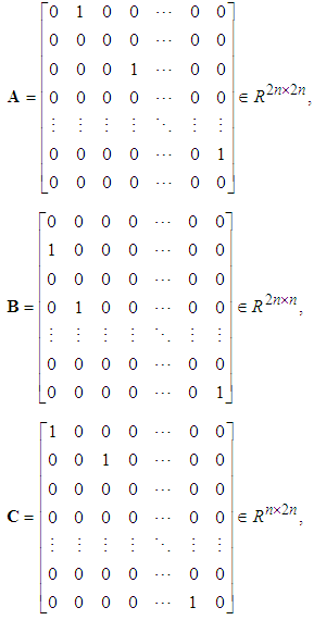
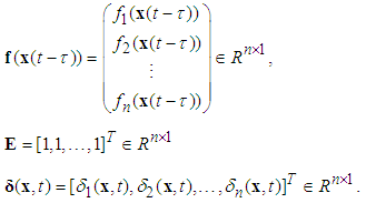
Consider a class of single-input multi-output uncertain underactuated nonlinear systems with time delay and dead- zone input expressed as follows:

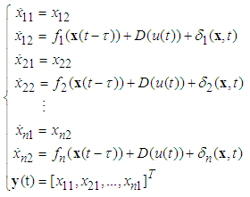(1)

where is the system state vector which is assumed to be unavailable for measurement, and are the input and output of the system, respectively. is the value of time delay , 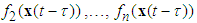are unknown real continuous nonlinear functions, and 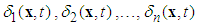are the unknown bounded disturbances. is the nonlinear input function containing a dead zone.

Assumption 1: The time delay is a fixed and known positive constant.

System (1) can be rewritten as

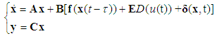(2)

where

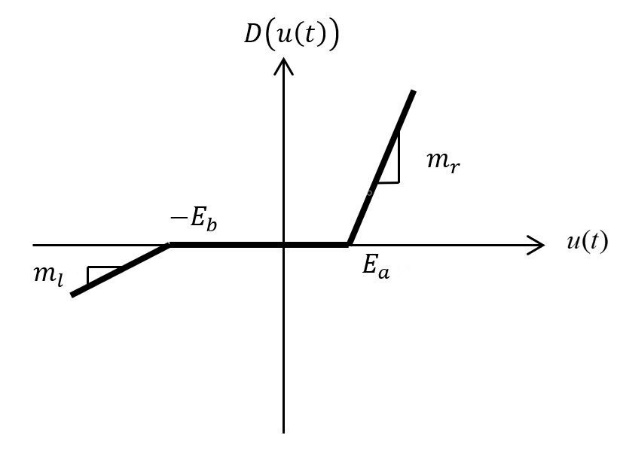Figure 1. Dead-zone model

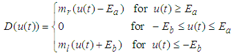(3)

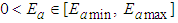
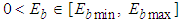
where and are parameters and slopes of the dead zone, respectively.

To investigate the key features of the dead zone in the control problems, the following common assumptions are given.

Assumption 2: The dead-zone output is not available to obtain.

Assumption 3: The coefficients and are unknown.

Assumption 4: There exist known constants and such that the unknown dead-zone parameters and are bounded, i.e. , , .

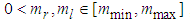Based on the above assumptions, the expression (3) can be rewritten as

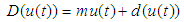(4)

where can be calculated from (3) and (4) as

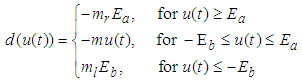(5)

From Assumption 4, it can be concluded that is bounded, and satisfies:

(6)

where is the upper bound, which can be chosen as

(7)

Assumption 5: , where h is an unknown constant.

Control objective: The control objective is to design a robust adaptive fuzzy controller to ensure that all the closed-loop signals are bounded.

2.2. Description of Fuzzy Logic Systems

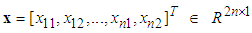
The fuzzy logic system performs a mapping from to. Let where , . The fuzzy rule base consists of a collection of fuzzy IF-THEN rules:

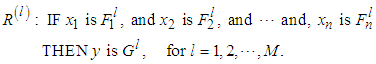(8)

in which and are the input and output of the fuzzy logic system, and are fuzzy sets in and , respectively. The fuzzifier maps a crisp point into a fuzzy set in .

The fuzzy systems with center-average defuzzifier, product inference and singleton fuzzifier are of the following form:

(9)

where with each variable as the point at which the fuzzy membership function of achieves the maximum value and with each variable as the fuzzy basis function defined as

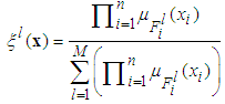(10)

where is the membership function of the fuzzy set.

3. Controller Design and Stability Analysis

3.1. Observer Design

First, the following fuzzy logic systems can be constructed, over a compact set , the unknown nonlinear functions can be approximated as

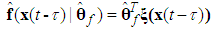(11)

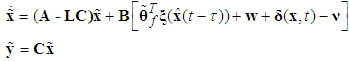
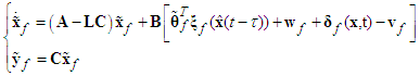
where is the fuzzy basis vector, is the corresponding adjustable parameter vector of the fuzzy logic system.

Because the system states are assumed to be unmeasurable in this paper, the fuzzy logic systems (11) cannot be directly used for the unknown nonlinear system. Therefore, an observer is designed to estimate the unmeasurable system states. Let us define that is the estimate of at first. Then, the following fuzzy logic systems can be obtained as

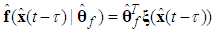(12)

The observer for system (2.2) is established as follows:

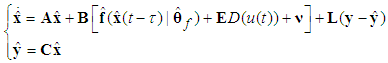(13)

where

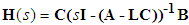
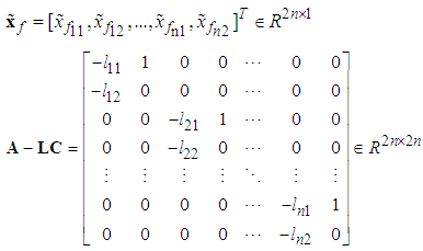
is the observer gain matrix to guarantee the characteristic polynomial of to be Hurwitz. The estimation error vector is defined as and , then according to (2) and (13), one has

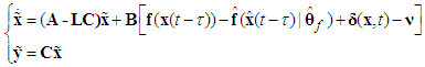(14)

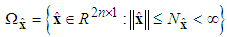
It is assumed that , and belong to compact sets , and respectively, which is defined as

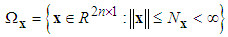(15)

(16)

(17)

where , and are the designed parameters, and M is the number of fuzzy inference rules. Let us define the optimal parameter vector as follows:

(18)

where is bounded in the suitable closed set .

The parameter estimation errors can be defined as

(19)

and

(20)

are the minimum approximation errors, which correspond to approximation errors obtained when optimal parameters are used.

According to (19) and (20), (14) can be written as

(21)

The output error dynamic of (21) can be expressed as follows:

(22)

where

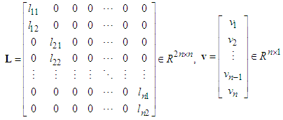
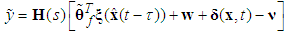
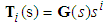
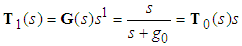
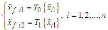
and s denotes the complex Laplace transform variable. As previously discussed in this chapter, not all elements of could be obtained, because not all the system states are available for measurement. Consequently, one could not obtain all elements of . The state variable filters [17] will be introduced to cope with this problem. The stable filter is chosen as follows:

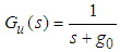(23)

for

(24)

Introducing (24) into (22), the steady-state equation can be written as

(25)

Define a set of state variable filters ,, thus,

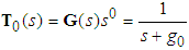(26)

(27)

The corresponding filtered signals are defined as follows:

(28)

(29)

(30)

(31)

(32)

Eq. (21) can be rewritten as follows:

(33)

where

It is assumed that there exists an unknown constant , such that

(34)

Let us define that

(35)

and

(36)

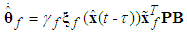
where and are the estimates of and h, respectively.

Based on Lyapunov stable theorem, the robust compensation term and the parameter update laws can be obtained as follows:

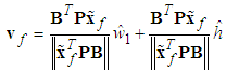(37)

(38)

(39)

(40)

where , , and are positive constants

Remark 1: Without loss of generality, the adaptive laws used in this paper are assumed that the parameter vectors are within the constraint sets or on the boundaries of the constraint sets but moving toward the inside of the constraint sets. If the parameter vectors are on the boundaries of the constraint sets but moving toward the outside of the constraint sets, we must use the projection algorithm to modify the adaptive laws such that the parameter vectors will remain inside of the constraint sets. Readers can refer to reference [16]. The proposed adaptive law (38) can be modified as the following form:

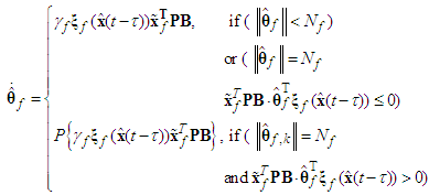(41)

where is defined as

(42)

The main result of the proposed robust adaptive fuzzy observer method is summarized on the following theorem.

Theorem 1: Consider the single-input multi-output uncertain underactuated system with time delay and dead-zone input (1). The robust adaptive fuzzy observer is defined by (13) with adaptation laws given by (37)-(40). For the given positive definite matrix , if there exists a symmetric positive definite matrix such that the following Lyapunov equation

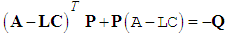(43)

is satisfied, then all the closed-loop signals are bounded, and the estimation errors converge to a neighborhood of zero.

Proof: Consider the Lyapunov function candidate

(44)

By the time derivate of and the facts 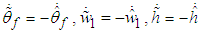one has

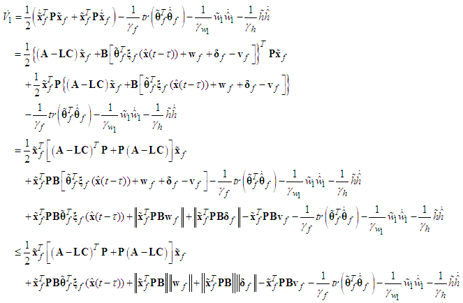(45)

Applying Assumption 5 and (34)-(36), one gets

(46)

Substituting (38)-(40) into (46), one obtains

(47)

Considering the robust compensation term (37), the above equation can be rewritten as

(48)

According to (43), it can be easily shown that

(49)

Therefore, it can be concluded that from (49), and the estimation errors of the closed-loop system converges asymptotically to a neighborhood of zero based on Lyapunov synthesis approach. This completes the proof.

3.2. Controller Design

Based on Lyapunov stable theorem, the observer-based controller is given by

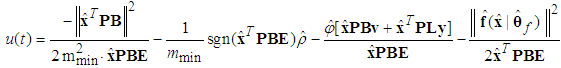(50)

Let us define the estimation error as

(51)

(52)

where is the estimate of , which is defined as . is the estimate of . The parameter update laws are as follows:

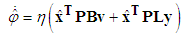(53)

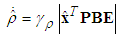(54)

where the scalar and are positive constants, and can be obtained by backward from .

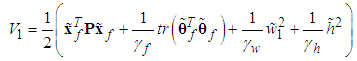
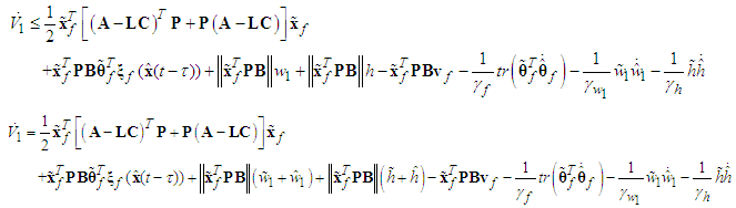
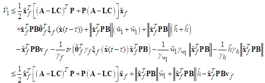
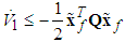
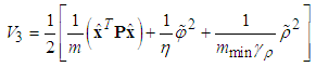
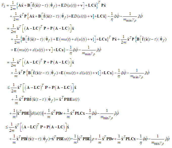
Theorem 2: Consider the single-input multi-output uncertain underactuated system with time delay and dead-zone input (1). The proposed observed-based robust adaptive fuzzy controller defined by (50) guarantees that all signals of the closed-loop system are bounded and converge to a neighborhood of zero.

Proof: Consider the Lyapunov function candidate

(55)

where

(56)

(57)

Taking the time derivate of and the facts yields

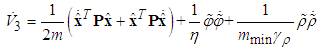(58)

Substituting (13) into (58), one has

(59)

By the inequality , Eq. (59) can be rewritten as

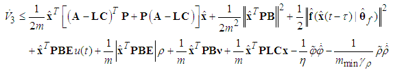(60)

Differentiating the with respect to time, one gets

(61)

With (60) and (61), according to the equation , one has

(62)

According to and Assumption 4, Eq. (3.54) becomes

(63)

Applying adaptive laws (53) and (54), yields

(64)

Using the controller (50), the above equation can be rewritten as

(65)

According to (43), it can be easily shown that

(66)

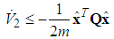
Therefore, it can be concluded that from (66), and the all signals of the closed-loop system converge asymptotically to a neighborhood of zero based on the Lyapunov synthesis approach. This completes the proof.

Remark 2: Because the discontinuities in the control term (50) give rise to chatter in the system, it has been proposed thatwill be replaced by a continuous approximation in an -width region of . Thus, replacingwith in (50), the is described by

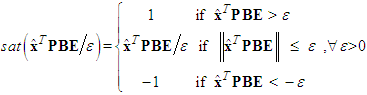(67)

Remark 3: The schematic diagram of the proposed control system can be delineated as shown in Fig. 2.

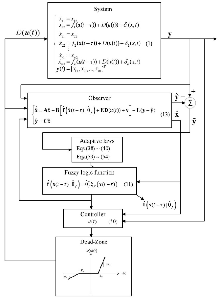Figure 2. The block diagram of the proposed control system

4. An Example and Simulation Results

In this section, a series of simulation results of a underactuated nonlinear system and a underactuated mass-spring-damper system are used to demonstrate the effectiveness of the proposed controller.

Example 1: An Underactuated Nonlinear System

Consider the underactuated nonlinear system:

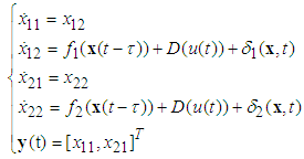(68)

where are the displacements of the masses. are the velocities of the masses.

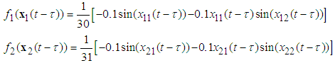
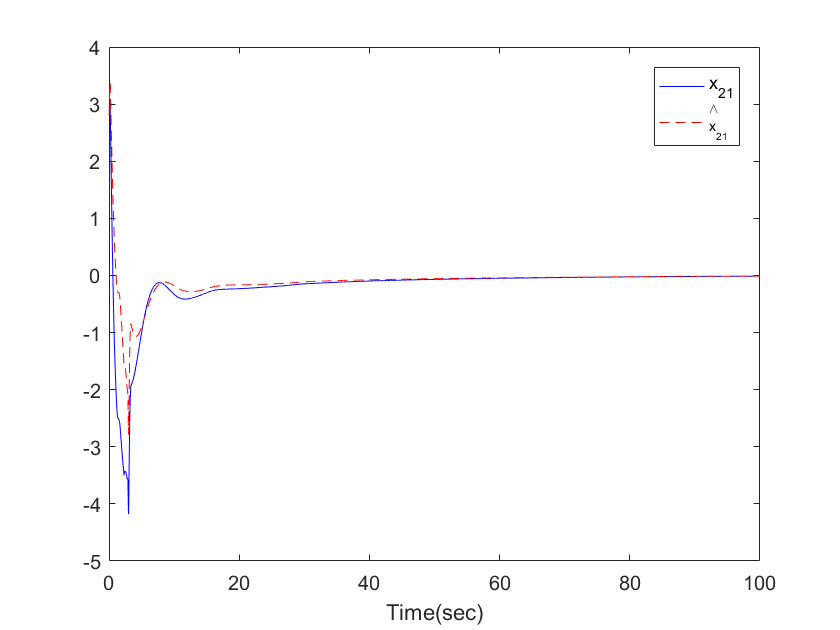
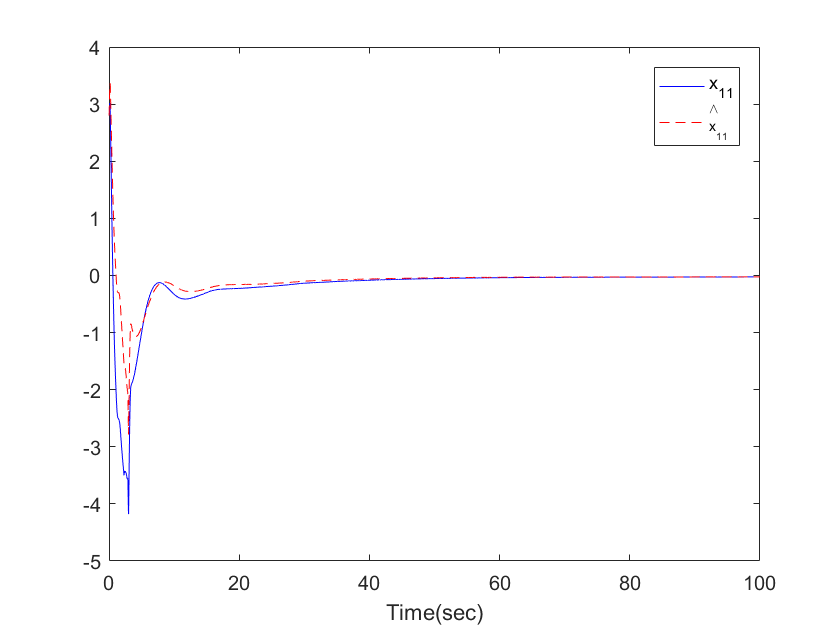Figure 3. The trajectories of and for Example 1

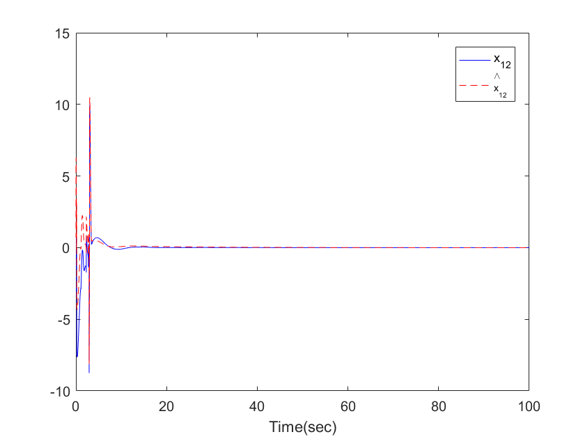Figure 4. The trajectories of and for Example 1

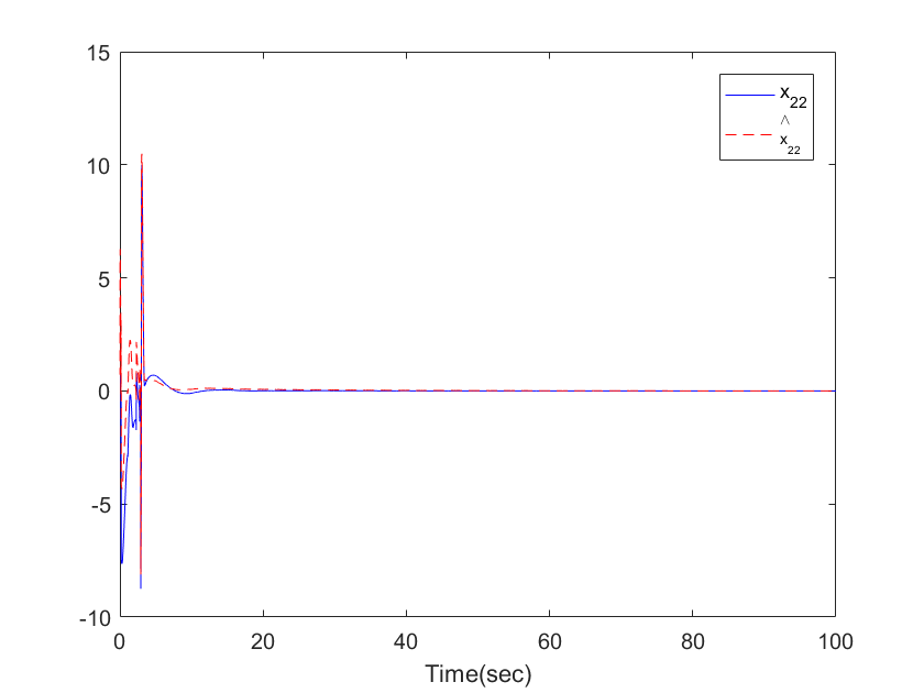
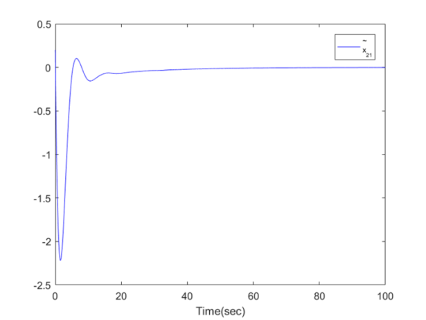
Figure 5. The trajectories of and for Example 1

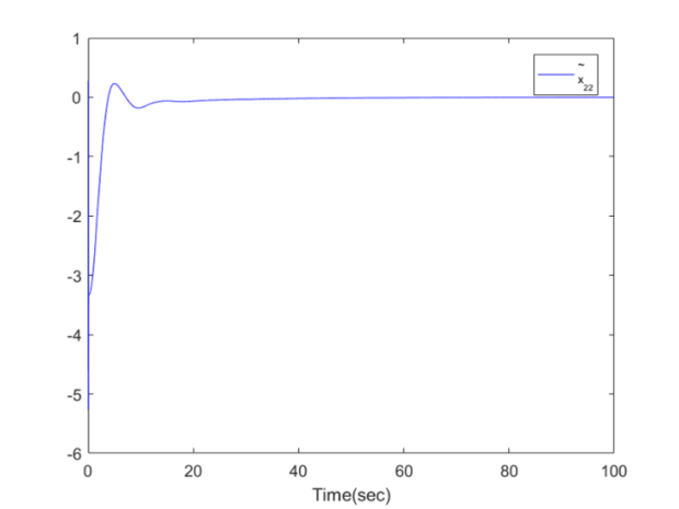
Figure 6. The trajectories of and for Example 1

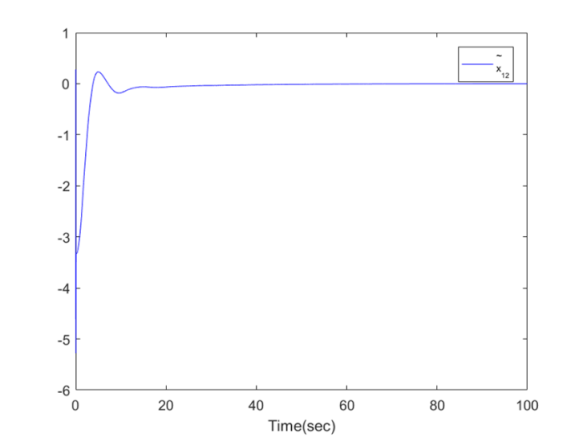
Figure 7. The trajectory of for Example 1

Figure 8. The trajectory of for Example 1

Figure 9. The trajectory of for Example 1

Figure 10. The trajectory of for Example1

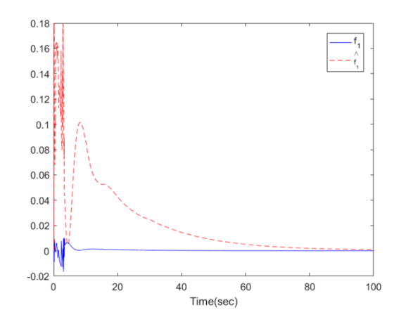Figure 11. The trajectories of and for Example 1

Figure 12. The trajectories of and for Example 1

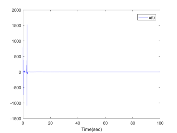Figure 13. The control signal for Example 1

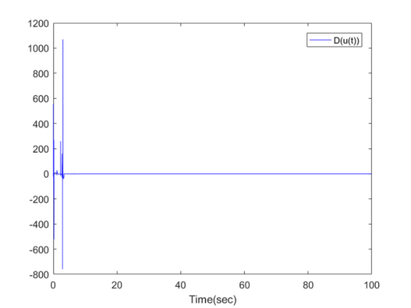Figure 14. The dead-zone input for Example 1

is an output of a dead zone, and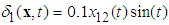, are the disturbances.

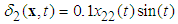
In the simulation, parameters of the dead zone are , , , . We select their bounds as , . Six fuzzy sets are defined over the interval [-3, 3] for , and , with labels NB, NM, NS, PS, PM, and PB, and their membership functions are

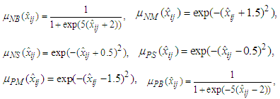where

Choose the sampling time as 0.01, and the observer gain as , , , . The initial values are chosen as , , , , , , , , , , , , , , . The other parameters are selected as , , , , , . The simulation results are displayed by Figs. 3-14. Figs. 3-6 show the trajectories of the system states and their estimation states. Figs. 7-10 show the trajectories of the system state estimation errors. Figs. 11-12 show the trajectories of the system functions. Figs. 13-14 show the trajectories of the control signal u and the dead-zone input .

5. Conclusions

An observer-based robust adaptive fuzzy control approach has been proposed in this paper for a class of uncertain underactuated systems in the presence of time delay and dead-zone input. The system states are assumed to be unmeasurable in this paper. With the help of fuzzy approximation, the fuzzy state observer has been constructed to estimate the unmeasurable states. Additionally, some adaptive laws are employed to estimate the unknown system parameters. The main contribution of this paper can be listed as follows: (i) the stability of the whole underactuated time-delay system has been proved via the Lyapunov-Krasovskii functional and (ii) all the signals of the closed-loop system are bounded by the presented control scheme. Finally, a series of simulation results have been presented to demonstrate the effectiveness of the proposed control approach.