1. Introduction

In recent years, switched systems have drawn much attention and some significant results have been obtained in the literature. As an important class of hybrid systems, switched systems can be described by a family of subsystems and a switching law between them. Actually, many practical systems, such as power electronic, automotive industry, mechanical systems, air traffic control, etc., can be expressed as switched systems [1-4]. Motivated by the above reasons, the control design and stability of the switched systems have received many researchers a great interest. In addition, dead-zone input nonlinearity is a nonsmooth function that features certain insensitivity for small control inputs which is often encountered in a variety of practical systems such as the single-link flexible joint manipulator, and so on [5, 17-18]. In this paper, the switched system in strict-feedback form is investigated and a feasible and systematic methodology is proposed to solve the tracking control problem.

Due to uncertainties inherent in practical systems, the design control capable of handling uncertainties is of practical interest and is challenging. To achieve the desired system performance, adaptive control is a valid methodology, which supplies adaptation mechanisms to regulate controllers for systems with some uncertainties, such as parametric, structural, and environmental uncertainties [6-7]. For non-switched nonlinear systems using fuzzy logic systems or neural networks to parameterise the unknown non-linearities, adaptive control of uncertain nonlinear systems has attracted much attention [8-9]. In recent years, adaptive fuzzy or neural backstepping approaches for strict-feedback form systems [10-11] provide some systematic methods to achieve good tracking performance.

Fuzzy logic systems (FLS) with appropriate adaptive laws algorithms are used to approximate the unknown nonlinear functions appearing in the structure of the switched system. A FLS consists of four parts: the knowledge base, the fuzzifier, the fuzzy inference engine working on fuzzy rules, and the defuzzifier. The problem of adaptive fuzzy output-feedback control for switched uncertain non-linear systems is investigated in [12, 19]. In [13], Li et al. introduced an adaptive fuzzy output-feedback stabilization controller to treat the problem for a class of switched nonstrict-feedback nonlinear systems.

Recently, sliding mode control (SMC) has been adopted as a powerful approach for the control of systems with external disturbances and parameter variations [14, 20]. Since SMC technique has some advantages, such as insensitivity to system parameter variations, invariance to external disturbances, good transient and fast response. Basically, SMC laws consist of two parts: switching controller design and equivalent controller design. The switching control law is employed to lead the system’s states to a given sliding surface and the equivalent control law guarantees the system’s states to stay on the aforementioned sliding surface and converge to zero along the sliding surface.

The main contribution of this paper is that the proposed SMC method deals with the problem of tracking performance and stability for a class of switched nonlinear systems in strict-feedback form with dead-zone input. Based on SMC technique, an adaptive fuzzy sliding mode controller is designed for the switched system by using fuzzy logic systems with some adaptive laws to approximate uncertain functions. The fuzzy state observer is employed to estimate the unavailable state for measurement. By choosing an appropriate Lyapunov function, it is theoretically ensured that all the signals in the closed-loop system are uniformly ultimately bounded and receive good tracking performance under our designed controller.

This paper organized as follows. Section II contains system description, dead-zone characterization, a detailed description systems, and fuzzy basis functions. Section III, the observer-based fuzzy sliding mode controller is utilized to treat the nonlinear switched system with dead-zone input. Simulation results are provided in Section IV to demonstrate the advantages and effectiveness of the proposed approaches Finally, the concluding remarks are gathered in Section V.

2. Problem Statement and Preliminaries

2.1. System Description

Consider a class of single-input-single-output switched uncertain nonlinear systems in strict-feedback form with dead-zone input expressed as follows:

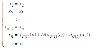(1)

where is the system state vector which is assumed to be available for measurement, and are the input and output of the system output, respectively. The function , is a switching signal which is assumed to be a piecewise continuous (from the right) function of time. If , then we say the kth switched subsystem is active and the remaining switched subsystems are inactive. is the unknown smooth nonlinear function, is unknown external bound disturbance. denotes the input function containing a dead-zone.

Then, the system (1) can be rewritten as

(2)

where

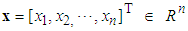
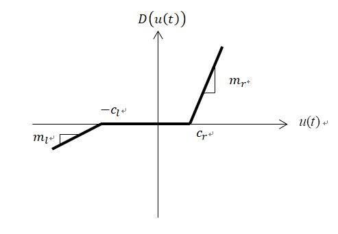Figure 1. Dead-zone model

The non-symmetric dead-zone with input and output as shown in the above Fig. 1 is described by

(3)

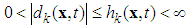
where, are parameters and slopes of the dead-zone, respectively. In order to investigate the key features of the dead-zone in the control problems, the following assumptions should be made:

Assumption 1: The dead-zone output is not available to obtain.

Assumption 2: The coefficients are unknown.

Assumption 3: The maximum and minimum values of the characteristic slopes are known. ,

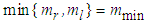Based on the above assumptions the expression (3) can be represented as

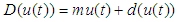(4)

where can be calculated form (3) and (4) as

(5)

From Assumption 1 and Assumption 2, we can conclude that is bounded, and satisfies:

(6)

where is an upper bound, which can be chosen as

(7)

Assumption 4：

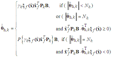
where is an unknown function.

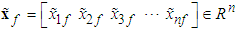
Control objective: Design a controller for (1) such that the system output y(t) would track the desired output vector , where be a given bounded desired signal and contain finite derivative up to the n order. Define the vector of the output tracking error as 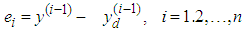. Thus,

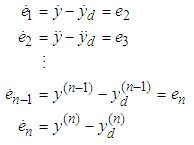(8)

2.2. Description of Fuzzy Logic Systems

The fuzzy logic system performs a mapping from to . Let where , . The fuzzy rule base consists of a collection of fuzzy IF-THEN rules:

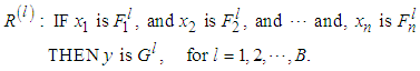(9)

in which and are the input and output of the fuzzy logic system, and are fuzzy sets in and , respectively. The fuzzifier maps a crisp point 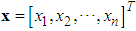into a fuzzy set in . The fuzzy inference engine performs a mapping from fuzzy sets in to fuzzy sets in , based upon the fuzzy IF-THEN rules in the fuzzy rule base and the compositional rule of inference. The defuzzifier maps a fuzzy set in to a crisp point in .

The fuzzy systems with center-average defuzzifier, product inference and singleton fuzzifier are of the following form:

(10)

where with each variable as the point at which the fuzzy membership function of achieves the maximum value and 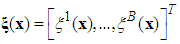with each variable as the fuzzy basis function defined as

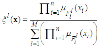(11)

where is the membership function of the fuzzy set.

3. Controller Design and Stability Analysis

3.1. Observer Design

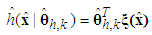
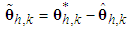
According to the description of the fuzzy logic system presented in Section 2.2, we can construct the following fuzzy logic systems, over a compact set, the unknown nonlinear functions and the uncertainty can be approximated as

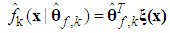(12)

(13)

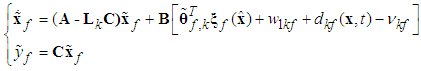
where is the fuzzy basic vector, and are the corresponding adjustable parameter vectors of each fuzzy logic systems.

Owing to the unavailable states of the system and the unavailable elements of the output error vector in many practical systems, the fuzzy logic systems (12) and (13) are not used to control nonlinear systems whose states are not obtained for measurement. Therefore, we must employ an observer to estimate. Let be the estimate of at first. Then, we can obtain the following fuzzy logic systems as

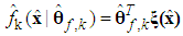(14)

(15)

In order to estimate the state, the observer can be chosen as follows:

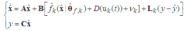(16)

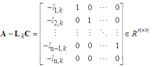
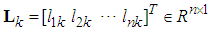where is the observer gain vector, and 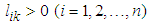are coefficients of the Hurwitz polynomial 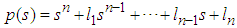. Define the estimation error vector as and .

Then from (2) and (16), we obtain

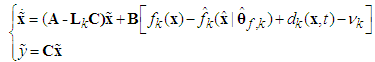(17)

It is assumed that and belong to compact sets 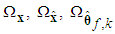and respectively, which is defined as

(18)

(19)

(20)

(21)

where are the designed parameters, and N is the number of fuzzy inference rules. Let us define the optimal parameter vector and as follows:

(22)

(23)

where and are bounded in the suitable closed set and . The parameter estimation errors can be defined as

(24)

(25)

Then,

(26)

(27)

are the minimum approximation errors, which correspond to approximation errors obtained when optimal parameters are used.

Applying (24) and (26) to (17), it yields

(28)

The output error dynamic of (28) can be expressed as follows:

(29)

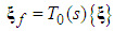
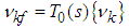
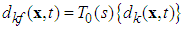
where and s denotes the complex Laplace transform variable. As has been discussed, we could not obtain all elements of , because not all states of the system are available or measurement. Hence, we could not obtain all elements of . We will employ the state variable filters [15] to cope with this problem. First, we choose a stable filter as the following form:

(30)

Where are coefficients of the Hurwitz polynomial .

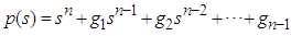Introducing (30) into (29), we can obtain the steady-state equation

(31)

Define a set of state variable filters as

(32)

The corresponding filtered signals are defined as follows:

(33)

(34)

(35)

(36)

(37)

Then, Eq. (28) can be rewritten as follows:

(38)

where

Define

(39)

where is the estimated of , and

(40)

Based on the Lyapunov stable theorem, we can obtain the robust compensation term and the parameter update laws as follows:

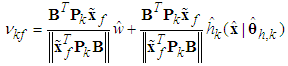(41)

(42)

(43)

(44)

where are positive constants

Remark 1: Without loss of generality, the adaptive laws used in this paper are assumed that the parameter vectors are within the constraint sets or on the boundaries of the constraint sets but moving toward the inside of the constraint sets. If the parameter vectors are on the boundaries of the constraint sets but moving toward the outside of the constraint sets, we have to use the projection algorithm to modify the adaptive laws such that the parameter vectors will remain inside of the constraint sets. Readers can refer to reference [16]. The proposed adaptive law (41)-(44) can be modified as the following form:

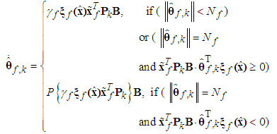(45)

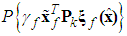where is defined as

(46)

(47)

where is defined as

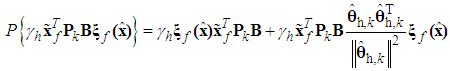(48)

The main result of the robust adaptive fuzzy observer scheme is summarized on the following theorem.

Theorem 1: Consider the single-input-single-output uncertain switched system in strict-feedback form (1). The robust adaptive fuzzy observer is defined by (16) with adaptation laws given by (41)-(44). For the given positive definite matrix, if there exist symmetric positive definite matrix such that the following Lyapunov equation

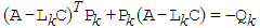(49)

is satisfied, then all signals of the closed-loop system are bounded, and the estimation errors converge to a neighborhood of zero.

Proof. Consider the Lyapunov function candidate

(50)

By the time derivate of and the facts 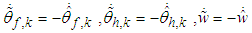we obtain

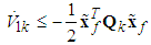
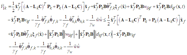(51)

Applying Assumption 4 and (27) and (40), it yields

(52)

By employing (42)-(44), we have

(53)

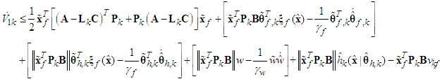
Then using the robust compensation term (41), the above equation can be rewritten as

(54)

According to (49), it can be easily shown that

(55)

Therefore, it can be concluded that from (55), and the estimation errors of the closed-loop system converge to a neighborhood of zero based on Lyapunov synpaper approach. This completes the proof.

3.2. Controller Design

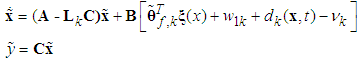
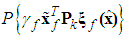
Next, we design the observer-based sliding mode controller. By employing (8) and (16), we get

Define the sliding surfaces as follows:

(56)

where is designed parameters.

Differentiating with respect to time, we have

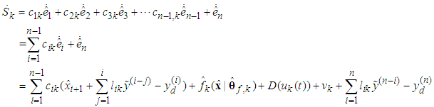(57)

Consider the following controller

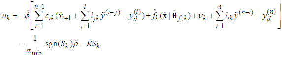(58)

in which is a positive constant, and is defined in (7).

We defined

(59)

(60)

where is the estimate of , which is defined as . is the estimate of . The parameter update laws are as follows:

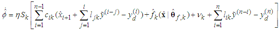(61)

(62)

where the scalar and are positive constants, and can be obtained by backward from .

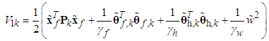
Theorem 2: Consider the nonlinear switched system (1) with an unknown dead-zone input (4). The proposed observed-based fuzzy sliding mode controller defined by (58) guarantees that all signals of the closed-loop system are bounded and converge to a neighborhood of zero.

Proof. Consider the Lyapunov function candidate

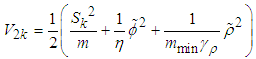(63)

Differentiating the Lyapunov function with the respect to time, we obtain

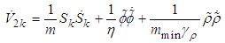(64)

By the fact and , the above equation becomes

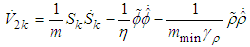(65)

Applying equation (57), equation (65) can be written as

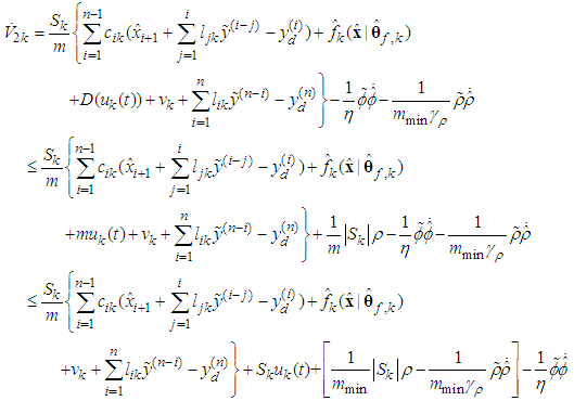(66)

According to , the above equation (66) becomes

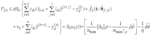(67)

Applying adaptive laws (61) and (62), we obtained

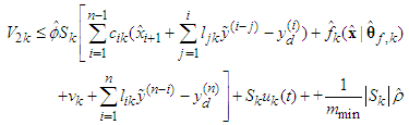(68)

Using the control law (58) the above equation can be rewritten as

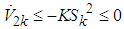(69)

Therefore, it can be concluded that from (69), and the all signals of the closed-loop system converge asymptotically to a neighborhood of zero based on the Lyapunov synthesis approach. This completes the proof.

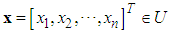
4. An Example and Simulation Results

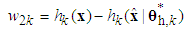
In this section, a mass-spring-damper system [12] in the presence of uncertain parameter and exogenous disturbances is considered as our simulation example in Fig. 2. The corresponding mathematical model is described as follows:

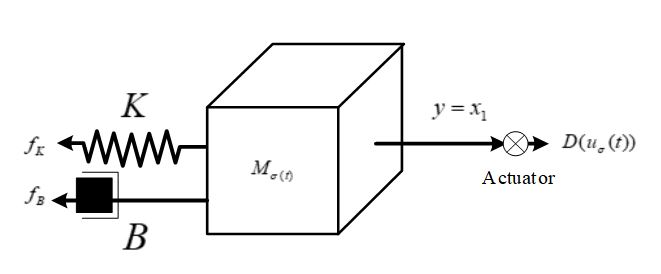Figure 2. The mass-spring-damper system

where is the displacement of the mass, is the velocity of the mass, are the spring force, , are the friction force, is the switched signal, and , is the body mass, and is the applied force. The structures of spring force and friction force are assumed to be known. The exogenous disturbance is assumed to be and , In the implementation, five fuzzy sets are defined over interval [-3,3] for , with labels and their membership functions are

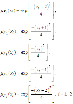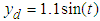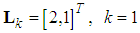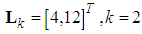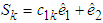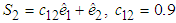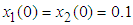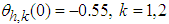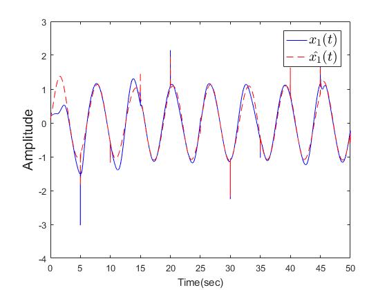
In this section, the control objective is to maintain the system output to follow the reference signal . First, we select the observer gain matrix as and . In this example, the sampling time is 0.01s. The sliding surface are select as . when k=1 , and when k = 2 . The initial values are chosen as , ,, . The other parameters are selected as , , and , . The simulation is divided into two cases, one for the dwell time of 5 seconds and the other for the dwell time of 1 second. Finally, the simulation results are shown in Figs. 3-12.

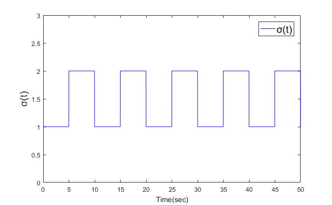Figure 3. The switched signal with dwell time is 5secs

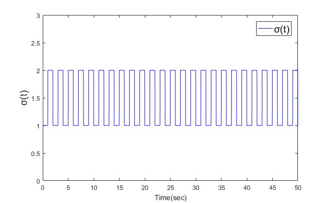Figure 4. The switched signal with dwell time is 1sec

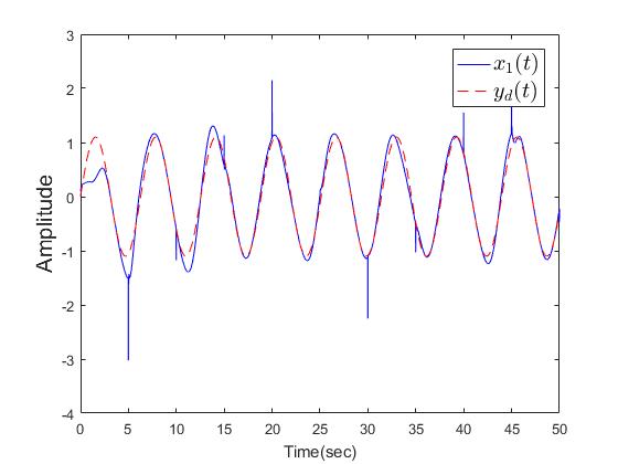Figure 5. The outputs with dwell time is 5secs

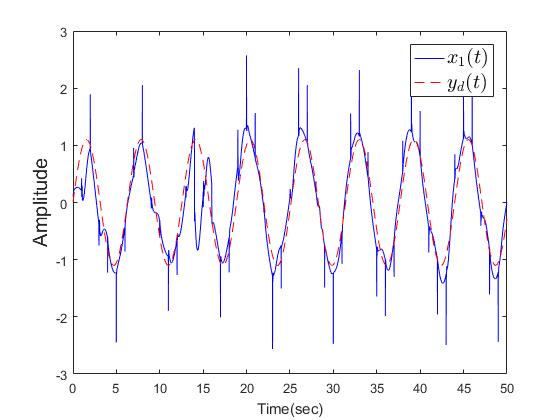Figure 6. The outputs with dwell time is 1sec

Figure 7. The trajectories of with dwell time is 5secs

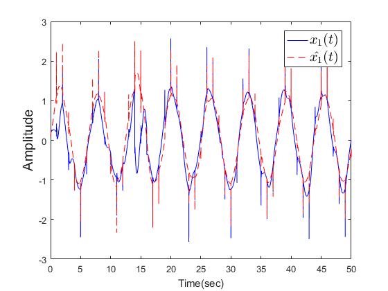Figure 8. The trajectories of with dwell time is 1sec

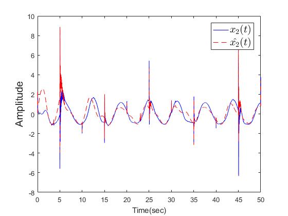Figure 9. The trajectories of with dwell time is 5secs

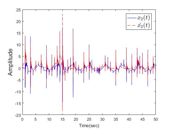Figure 10. The trajectories of with dwell time is 1sec

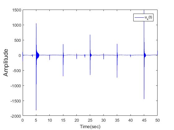Figure 11. The control signal with dwell time is 5secs

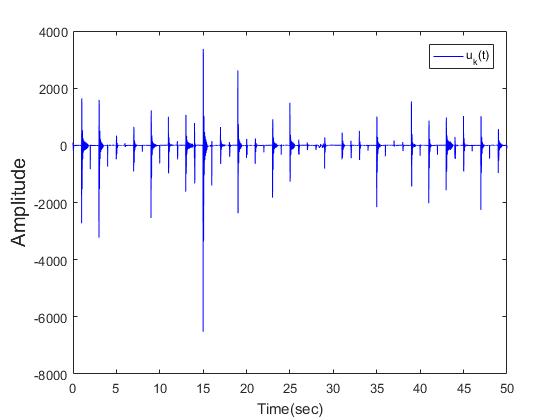Figure 12. The control signal with dwell time is 1sec

Remark 2: According to the above simulation results, it can be found that if the dwell time of the system is longer, then the system tracking performance is better, and if the dwell time of the system is shorter, then the system cannot achieve good tracking performance.

5. Conclusions

An observer-based adaptive fuzzy sliding mode control approach has been proposed for a class of uncertain switched nonlinear systems with dead-zone input in strict-feedback form. A fuzzy state observer has been designed for estimating the unavailable states with the help of FLS approximating the unknown functions. Based on the designed sliding mode controller, the boundedness of the proposed sliding surfaces which realizes the stability of system can be ensured. By choosing an appropriate Lyapunov function, the proposed controller is designed to demonstrate that all the signals of the closed-loop system can not only guarantee uniformly ultimately bounded, but also achieve good tracking performance. Finally, some computer simulation results of a practical example are illustrated to verify the effectiveness of the proposed approach.