1. Introduction

Ore milling is one of the primary operations in mineral processing and it is known to account for approximately half of all costs in a mine, largely attributable to energy and material expenditure [3]. A key strategy for achieving lower energy and material costs in ore milling circuits is through effective mill control [10, 13]. However, such a control system would require good understanding of the in-mill dynamics when the operating variables are changed and the interactions between external process variables and performance variables. Indeed grinding mills in mineral processing plants never really operate under steady state conditions as variations in feed size distributions, feed rate, feed slurry density and ore characteristics continuously upset the smooth running process.

Today, PID (proportional-integral-derivative) controllers are the common computational based online control schemes. However, they are tuned to work for only a known set of operating conditions (incapable of self-tuning) and preferably for systems with non-interactive variables. If there is a change in these system conditions, the tuning parameters become less suitable. In a milling circuit, if a given mass setting of the mill creates poor mill performance, then a new mass set-point will have to be established in order to maximize mill performance. Such a development in the mill circuit cannot be recognized by a PID controller, which implies that on its own, a PID controller cannot optimally control a grinding circuit. Recent years have seen development of expert control systems to address this need. The expert control system allows for interaction to correct for deviances, and optimal values for set-points. Thus, the expert control system relies on understanding of the process and the dynamic characteristics of many critical variables around the process.

Better understanding of the in-mill dynamics can be gained in a much faster and economical manner through dynamic simulations (on-line or off-line) using accurate mill simulation models. Prior insights into the behaviour of the milling circuit can be made available such as response to grinding process disturbances during transitions between various steady-states. Also, the multivariable interactions within the mill circuit can be easily explored and evaluated and changes can then be made to the circuit to realise better efficiency and high throughput at lower costs. This inherent flexibility, coupled with robustness makes model-based control approach more advantageous in today’s highly integrated and complex comminution circuits.

The fundamental aspects required for accurate dynamic simulation are good dynamic models, precise measurements of process variables and accurate estimation procedures for process parameters [8, 9, 18]. A range of simulation models exist, which have been widely used for mill circuit design and optimization with varying levels of success. But these models do not consider the energy balance inside the mill and are mainly based on steady state analysis. Apart from mass and size balance, energy balance is a key aspect in control and optimization of a comminution process. Energy balance data is related to mill temperature where the latter is believed to be a primary indicator of in-mill process dynamics [21, 12].

It is a known fact that the biggest part of energy introduced in a ball mill is converted into heat, with only about 3 - 5% of this energy being used to grind the ore to the required fineness. As a consequence, this heat induces temperature rise inside the mill. Therefore, interpretation of the temperature signature would yield some useful information of the mill operation characteristics such as variations in feed rate, slurry properties, holdup mass and degree of mixing inside the mill which are directly linked to grinding process. Having the knowledge of these dynamics enables effective control of the grinding mill which in turn results in stable operation with optimum production capacity and energy efficiency. It is noteworthy that temperature measurements can be made quite easily and far more accurately than other process measurements in a milling circuit.

This research aims to develop a dynamic model of mill temperature that may be employed alongside the conventional control system to provide indications of changes in mill operational characteristics. The model is developed in MATLAB environment, integrating the energy balance with the population balance in a simple and clear representation of the physics and thermodynamics of a wet ball milling process. The control parameters are mill power and product size distribution which are easily measurable. The success of this modelling technique would go alongside improving the continuous optimization and control of grinding mills.

2. Model Development

2.1. Model Framework

A dynamic model is developed for a wet overflow ball mill based on a set of mass and energy balances. The energy balance relies on temperature and mass flow data. The key model parameters to be measured are mill temperature in the feed and discharge streams, mill power draw and the mass flow rate in the feed stream. Manipulated variables are feed size distribution, feed solids concentration and flowrate of mill feed dilution water. Figure 1 is a schematic representation of the energy and mass flow streams around the mill operating in an open circuit configuration.

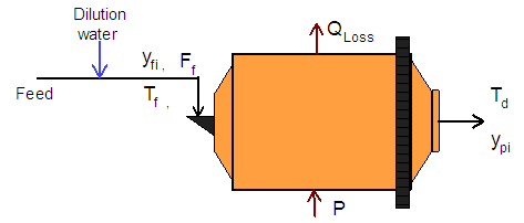Figure 1. Representation of mass and energy streams around the mill

Where, P is the power input (kW) to the mill, F_f is the feed flow rate into the mill (fresh feed + dilution water), T_f is the temperature of the mill feed, T_d is the temperature of mill discharge, Q_Loss is the rate of energy loss to the environment (kJ/s), y_fi is the mass fraction of mill feed solids in size class i while y_pi is the mass fraction of mill product solids in size class i.

Figure 2 is the conceptual framework of the model which depicts the mill as system of N perfectly mixed cells of equal volume, V with a net volumetric flow rate, F_f and recirculation rate, F_b. The total flow rate through stages 1 and N is F_f + F_b while the flow rate through stages 2 to N-1 is F_f + 2F_b. The set of equations which describes the dynamics of the system can be obtained by performing a material balance. The temperature of the mill discharge is assumed to be equal to the temperature in the last mixer and so is the slurry solids concentration.

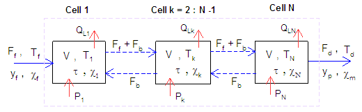Figure 2. Depiction of mass and energy streams in a mill represented by 4 equally sized and fully mixed segments with back-mixing

The model inputs are: breakage function parameters, selection function parameters, mill feed rate, mill dilution water, feed solids concentration, feed size distribution, mill rotational speed and mill level of filling. The outputs variables are the mill discharge temperature and the product size distribution.

2.2. Energy Balance

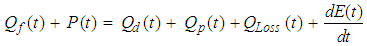
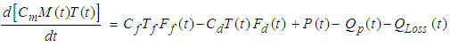
According to the fundamental laws of physics, the energy profile within a body depends upon the rate of energy input including internal generation, its capacity to store some of the energy and the rate of energy transfer to the surrounding environment i.e. Energy input = Energy output + Energy accumulation. Considering a wet ball mill operating in a continuous mode, then this equation can be expressed as follows:

(1)

Where Q_f is the rate of energy input through the feed stream while P represents the mill power input. Q_Loss represents the energy loss per unit time which comprises losses through conduction, convection, vapour, sound and vibration while Q_d is the rate of energy loss through the discharge stream. The term Q_p represents the energy absorbed per unit time by the particles to cause fracture, which is a function of material properties and mill conditions [16, 17]. Typically Q_p is so small relative to the total energy input to the mill, that it cannot be reliably measured. Since the model will be tested against data obtained on a full scale mill, some simplifying assumptions are considered in the energy balance. The assumptions are as follows:

i) That all the net power supplied to the mill, is transmitted to the mill charge as frictional energy at the grinding zones where part of it is converted to heat and lost to the environment through mill discharge product and vapour with the rest being lost in form of sound and vibration.

ii) That the mill contents are well mixed both in the radial and axial directions.

iii) That the slurry and grinding media in the mill are at thermal equilibrium and that the reference enthalpy of water and solids is zero at 0°C.

The overall dynamic energy balance around the mill can then be presented as equation 2 in which M(t) is the slurry holdup mass inside the mill approximated as,

(2)

The value of C (specific heat capacity of slurry) varies with the proportion of solids (χ) in the slurry and can be estimated by equation 3 in which the C_s and C_w denote specific heat capacity of solids and water respectively.

(3)

The rate of energy loss through sound and vibration is typically small relative to the net energy input into the mill, hence it could be neglected. Also, for mills fitted with rubber liners like the one used in the current study, energy loss through convection and conduction is minimal and hence can be ignored. A significant proportion of the energy loss to the environment will occur through evaporation (i.e. heat loss through vapour at the feed and discharge openings) which has to be accounted for. Therefore besides the temperature measurements, the prediction accuracy of this model will depend on correct estimation of Q_Loss and Q_p. Using standard bond work index, Q_p is estimated to lie between 1- 3% of the net energy input to the mill [7, 19] depending on ore characteristics (hardness and size). Thus, in this study, Q_p is modeled as a linear function of the net mill power draw in the form, . 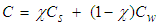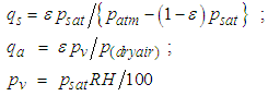It is worth to note that mill power can easily be measured using mill supervisory and data acquisition (SCADA) system and is expected to vary with changes in mill filling, feed size distribution and slurry properties.

The rate of energy loss from the mill through water vapour is a function of in-mill temperature, the humidity of the air overlaying the mill load and the slurry-air interfacial area where the latter is related to the size of the slurry pool. Thus, Q_Loss can be estimated by the following relation.

(4)

Where λ_L (kJ/kg) is the latent heat of vapourization, estimated empirically as λ_L = 2501 – 2.361T [5], ρ is the density of overlaying air, L_m is the mill length, J is the mill filling (J_max is dependent on the size of the discharge trunnion), D_m is the mill diameter while K_v is a correction parameter whose value is to be estimated and is related to the volume of vapour generated. The parameters q_s and q_a represent the specific humidity of air overlaying the load at saturated and unsaturated states respectively which are determined by equation 5 in which, ε (= 0.622) is the ratio of molecular weight of water vapour to that of dry air and RH is the relative humidity (%) at temperature, T [14].

(5)

Where,

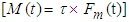
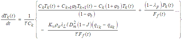
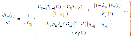
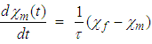
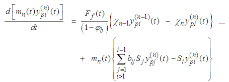
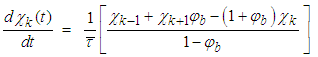
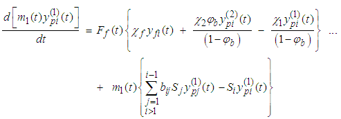
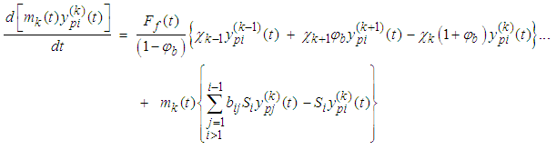
The residence time (τ) has been correlated to the feed percent solids in the form, (τ = K₁χ_f + K₂J), [11]. Here, K₁ and K₂ are constants to be determined by regression while J is the fraction of mill filling. Performing an energy balance around the mill system represented by n-mixers (Figure 2), yields equations that describe the temperature variation with time inside the mill. The symbols and represent the length and residence time of a single mixer respectively while (φ_b) is the back-mixing coefficient which is related to the axial dispersion coefficient.

Mixer 1:

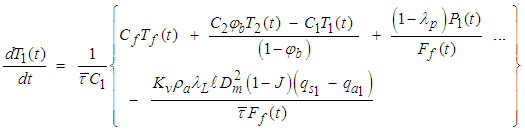(6a)

Mixer k = 2 to n-1

(6b)

Mixer n:

(6c)

The values of the back-mixing coefficient (φ_b) lie between 0 (no mixing) and 1 (perfectly mixed state). This parameter is a strong function of slurry solids concentration and could be estimated by the relation, (φ_b = K_A + K_B/χ_f) [11], where k_A and k_B are obtained by regression.

2.3. Mass – Size Balance

The size-mass balance is developed with reference to the mill system in Figure 1. Applying the principle of mass conservation to the milling process, the rate of accumulation of material of size i = rate of entry of material of size i from the feed + entry of material of size i from breakage of larger sizes - material destroyed in size i by fracture - disappearance of material of size i through discharge. This can be mathematically represented by the following steady state equation.

(7)

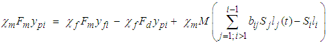
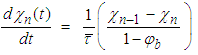
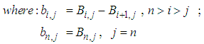The parameters b and S are the breakage distribution function and the selection function respectively that can be obtained using equations proposed by Austin et al [1], while F_m, χ_m and χ_f denote the mass flow rate through the mill and the slurry solids fraction inside the mill and in the feed stream respectively. The rest of the parameters retain their earlier definitions. For a well-mixed mill, the size of particles inside the mill would be equal to the mill product size (l_i = y_pi) and the average residence time would be given by the relation, (τ = M/F_m).

The population balance equation presented in Literature [1, 6] for determining the selection function characterizes particles only by their sizes. However, it is well recognized that the mechanical properties of brittle materials such as mineral bearing ore rocks strongly depend on deformation rate and strain rate. Therefore in population balance modelling of particle breakage process, the selection function should allow for particles to be characterized simultaneously by their size and fracture energy. The function should comprise the probability of a particle being selected for breakage and the probability of the energies generated by the impacts being sufficient to break the particles.

According to the work by Crespo [2], the probability of the energy applied being sufficient to break the particle is related to the fraction of the absorbed impact energies in a given time interval that are higher than the fracture energy. Similar observations were made by Tugcan and Rajamani [20] in a separate study using ultra-fast load cell data, who further indicated the dependence of this probability on particle size and material specific properties. For instance, a material with a higher hardness index would store more strain energy during deformation hence depending on the level of applied strain, it may require repeated impacts to fracture a hard material. This observation is supported by the data from Discrete Element Method (DEM) [4, 15], which shows that the impact frequency inside the mill depends on the level of energy applied. Due to lack of appropriate data on fracture energies of various mineral ore rocks, the size dependent rate of particle fracture shall be adopted in our model. From equation 7, the dynamic mass-size balance model can be written as follows:

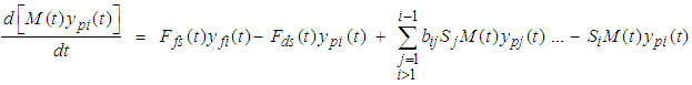(8)

The vectors, y_pi(t) = [y_p1(t), y_p2(t), … y_pn(t)]^T and y_fi = [y_f1, y_f2, … y_fm]^T represent the mass fraction of solids in the mill product and mill feed respectively in discrete size classes while F_fs (= χ_f F_f) and F_ds (= χ_m F_d) are the mass flow rates of the solids in the feed and discharge streams respectively. For overflow mills, typical of the one used in this study, the volume of slurry present in the mill is reasonably constant over a wide range of operating conditions, hence the volumetric feed rate to the mill equals volumetric discharge rate at all times. Utilizing this fact, the variation in proportion of solids in slurry, defined here as the mass of solids per unit mass of slurry in the mill, can be described by the following equation.

(9)

Similarly to the energy balance, the size-mass balance is performed with reference to the mill system presented in Figure 1. The superscripts in the brackets denote the mixing cell number i.e. k = 1 to n where n is the total number of mixing cells considered.

Mixer 1:

(10a)

Mixer k = 2 to n-1:

(10b)

Mixer n:

(10c)

The mass holdup of solids in each individual mixer at any time instant is dependent on; the level of solids concentration in the mixer, the mass feed rate and the residence time of the individual mixer as follows:

.

It is expected that the variation in slurry solids concentration between mill cells (m_1, m_k and m_n) would be marginal due to back-mixing effect. Performing the solids balance around the n mixers, we obtain the following equations representing the dynamic variation of solids concentration in each respective mixer.

Mixer 1:

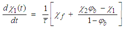(11a)

Mixer k = 2 to n-1:

(11b)

Mixer n:

(11c)

The task of mass and energy balancing has been accomplished numerically using MATLAB ode45 solver.

3. Results and Discussion

3.1. Experimental Data

Experimental data utilized in this research was obtained from an industrial secondary ball mill at Anglo-Platinum concentrator plant in South Africa at typical operating conditions. The mill measured 7.3 m diameter by 9.6 m long. Under normal operating conditions, the mill ball filling is 30% of total mill volume, mill speed is 75% of critical speed, solids concentration in slurry is 75%, solids feed rate is 330 tph and rated power draw is 9500 KW. Figures 3 and 4 present the trends in the data for 14 experimental surveys conducted at varying conditions.

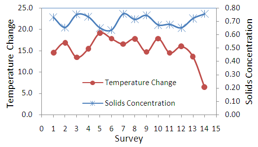Figure 3. Trends of mill temperature change and slurry solids concentration for 14 surveys conducted on an industrial mill

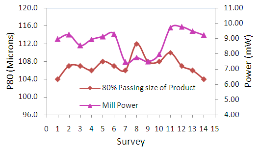Figure 4. Trends of mill power draw and product size (P80) for 14 surveys conducted on an industrial mill

A systematic pattern is clearly displayed in the trends of slurry solids concentration and mill temperature changes. Increasing the solids concentration tends to suppress the temperature gradient. This trend could be attributable to improved mixing inside the mill at higher solids concentration. This observation points to an available possibility of using information contained in mill temperature profile to track the evolution of slurry solids loading inside the mill. A consistent trend is also noticeable between the mill power draw and mill product size (P₈₀), which are efficiency indicators of a milling process. The P₈₀ is finer at higher mill power and vice versa which is consistent with the experience in milling practice. However, as solids concentration is increased, the mill power reduces. This is because the mass of the slurry pool in the mill (which exerts a torque counter to the torque drawn by the load) increases more rapidly than the mass of slurry in the load.

3.2. Steady State Tests

A total of 14 tests were conducted on a full scale ball mill at different steady states to allow measurements of mill temperature change between the feed and discharge points. The steady state set points were as follows: Load filling of 0.25, 0.3, 0.33 of total mill volume and slurry solids concentration of 65%, 67%, 70%, 72% and 75%. The results obtained were compared with model predictions as shown in Figure 5. The model describes the experimental data fairly well at steady state conditions.

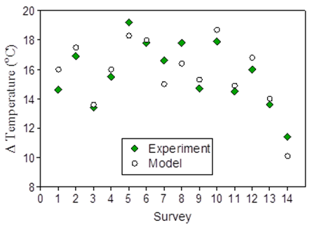Figure 5. Comparison of measured versus model predictions of mill temperature changes for 14 surveys conducted on an industrial mill

3.3. Dynamic Response Tests

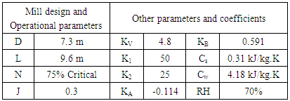
Test results of the model showing dynamic response of mill temperature to step changes in slurry solids concentration are shown in Figure 6. The corresponding results of the mill product size distribution for 30 minutes of milling are presented in Figure 7. The parameters used in the model are presented in Tables 1 and 2. The mill parameters are entered into the model simulator interactively using a simple user interface.

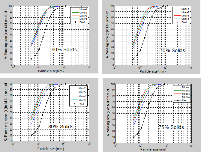Figure 6. Simulated particle size distribution of the mill product after 30 minutes of milling

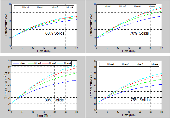Figure 7. Simulated in-mill temperatures for 30 minutes of milling at different levels of slurry solids concentration

Table 1. Model parameters

Table 2. Breakage and selection functions parameters

The results in Figure 6 show that the mill product is finer at higher solids concentrations of 75 and 80%. We believe that at higher proportion of solids, the slurry viscosity and particle packing is increased which enhances the friction within the mill load thereby strengthening the load lifting action, consequently improving the grinding. Also, the high energy impacts that result from high lifting action generate more heat which induce temperature rise. This explains the observed trends in Figure 7. Dilute slurry (lower solids concentration) tends to reduce friction within the load and cushions the ball impacts thus suppressing the grinding process.

3.4. Sensitivity Test

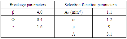
The sensitivity of temperature to variations in solids concentration and mill dilution water was assessed by the model. The mill simulation was run for 30 minutes (measured residence time) at each steady state before introducing a step change in the feed solids concentration by adjusting the mass flowrate of dilution water. The total simulation time was 90 min for the 3 levels of solids concentration utilized.

The profile of temperature changes correspond well with variations in slurry solids concentration and mill dilution water as demonstrated by the results in Figure 8, but only from a qualitative approach. Changes in mill temperature coincide with changes in solids concentration as feed dilution water is adjusted. Addition of dilution water results in negative change in temperature. These trends clearly indicate the sensitivity of temperature to perturbations in the slurry solids concentration. Thus, the evolution of slurry solids concentration inside the mill can be well traced using temperature profile.

Figure 8(a, b, c). Profile of mill temperature change with variations in feed solids concentration and mill dilution water

4. Conclusions

A simple dynamic model combining energy, mass and population balances has been utilized to assess the dynamic response of the mill to changes in mill operational parameters for purpose of establishing a predictive control tool. The manipulated parameters are solids feed rate, feed solids concentration and dilution water while the response variables are mill power draw, mill temperature and mill product size distribution (P₈₀). The results demonstrate a good dynamic response of the model to variations in mill operational parameters. Specifically, the profile of temperature changes inside the mill corresponds well to changes in mill slurry solids concentration. These observations justify the exploration for novel process control strategies that would enhance the effectiveness of mill control. The results assert the recommendations by previous researchers [13, 21] that temperature could provide significant insights into process behavior of a mineral processing unit which in turn may help to improve the control and optimization of the process. Once accurately calibrated, the temperature model can assist in providing early diagnosis of an ‘ailing’ mill that could be drifting off the desired operating curve.

ACKNOWLEDGEMENTS

The authors are grateful to Anglo-Platinum, South Africa for the financial support and providing the industrial mill data.