1. Introduction

Contemplating autonomously overcoming dynamic disturbances in space and unexpected changes in mass inertia may be addressed by the general methodology of deterministic artificial intelligence which stems from a lengthy heritage that harkens back at least 1830 with Chasle’s theorems of motion Phoronomics [1] followed shortly afterwards in 1846 with Newton’s Principia [2], continuing in 1775 with Euler’s formulations [3] with relatively immediate expansion throughout the nineteenth [4-7], justifying the later adopted of Tait angles to describe kinematics; and then followed in twentieth centuries [8-30] with a particular renaissance in the late twentieth century accompanying the race between the then-Soviet Union and the United States for spaceflight and its accompanying application toward nuclear deterrence, where considerable lessons from that period (both technical and non-technical) have been recently expressed in subsequent literature [31-69]. From this distinguished lineage, a contextual aspect has resurfaced with the rise of the looming threat of great power conflict in a context of many world powers also becoming space-faring nations. Accompanying this political context once again, the modern age sees impetus for significant technological advancement, this time towards autonomous, fault-tolerant, damage-tolerant control systems that include online state estimation, adaptive and non-adaptive feedforward controllers for trajectory tracking and disturbance rejection; and autonomous trajectory generation together forming intelligent space systems that no longer require phalanx’s of ground personnel to operate space systems. This article discusses recent research in the underlying technologies of rotational mechanics, modern kinematics (in an information-age context), and disturbance modeling for autonomous robust rejection, with particular emphasis on the italicized topics. From the recent literature, we see that [46-55] the deterministic artificial intelligence methodology can counter mass inertia disturbances up to 90% while maintaining single-digit to decimal degree accuracy [51] where this key metric will be used in a novel comparison of performance in a realistic disturbance environment amidst retention of significant mass vis-à-vis an apogee kick motor. Nonlinear stability is demonstrated via lyapunov-energy function in [39] and using phase portraits in [51].

2. Materials and Methods

2.1. Rotational Mechanics Fed by Autonomous Trajectory Generators

Initial modelling developed a commanded spacecraft body movement, and subsequently translates the commanded-movement into input torque commands applied to the spacecraft’s body. Kinematics subsystems expressed the quaternion and direction cosine matrix (direction cosine matrix) and used to find Euler Angles for attitude with respect to an inertial reference frame. The simulation topology of is shown in Figure 1.

Figure 1. Simulink Model Topology

The effects of varying time-steps and commanded maneuver-time in feedforward control (everything to the left of dynamics block in figure 1) are investigates, in particular emphasizing the numerical accuracy and impacts on computational time for various methods.

2.2. Dynamics

Dynamics is synonymous with Mechanics. Newton called dynamics the science of machines which may be divided into two parts: statics (later called kinematics) and kinetics [4]. Chasle’s Theorem [1] articulates how a complete description of motion may be described screw displacement comprised of translation in accordance with Newton’s Law and rotations in accordance with Euler’s Moment Equations 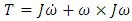[9] (both equations named subsequent to Chasle’s expression), where m is the mass of the object and [J] is a matrix of mass moments of inertia very well explained by Kane [24]. Thus, unplanned changes in the components of [J] are deleterious since the control force F applied as a torque is designed for the formerly assumed [J].

Investigation of motion without consideration of the nature of the body moved or how the motion is produced is called Phoronomics, or “the laws of going”, or more commonly but less properly kinematics [12], to be briefly discussed in section 2.3.

(1)

The Dynamics block of the system topology in Figure 1 contains equation (1) elaborated in equations (2) and (3), while the calculated command torque is provided by equation (4) in the Feed Forward Control section fed by equations (25)-(28) in the Trajectory Generator (the far left inputs of the topology) to be elaborated in section 2.4.

(2)

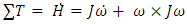
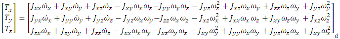
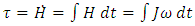
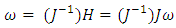
In the spacecraft’s dynamics captured in equation (1) and (2), represents the moment of inertia, is the angular velocity, and is the angular acceleration. In (2), the angular momentum, defined as H, with its change defined as . The additional component in equation (1) represents the coupled motion of the spacecraft when there is rotation about more than one axis. This coupling creates induced motion about the other axes and is proportional to the mass distribution in the inertia matrix.

To derive the angular velocity of the body fed from Dynamics to Kinematics, we multiply moment of inertia (J) by the time derivative of angular velocity, i.e., angular acceleration This term is multiplied by the inverse of J and then integrated as per equations 2 and 3. Afterwards, is used to obtain the spacecraft attitude’s Euler Angles.

(3)

Any change in Moment of Inertia will impact the ability of a spacecraft to execute commanded maneuvers. This paper studies the impact of a discrete change in moment of inertia on the ability of a numerically modeled (rigid body) spacecraft to successfully implement a commanded Euler angle maneuver. A sudden change in moment of inertia simulates large discrete changes, resulting from scenarios in which there are major changes to the spacecraft’s mass or mass distribution, such as orbital debris damage, jettison of a large component or stage, or catastrophic failure of major mass components. The model was used to simulate a single discrete change in the moment of inertia while implementing a 30° yaw maneuver.

Equation (4) contains the idealized feedforward control that forms the basis of deterministic artificial intelligence [66]. It is called idealized, because the control is formulated from equation 1 with moments of inertia assumed from the last known values, while the motion-states are provided by a desired tractor (thus the subscript d) in equation (4). This dependency also highlights the importance of the desired trajectory to be discussed in section 2.4.

(4)

Equation 4 is the foundational basis of deterministic artificial intelligence.

2.2.1. Change in Moment of Inertia

Change in the moment of inertia in the spacecraft is a common occurrence. Example scenarios include, the shifting of an internal component of a spacecraft during launch, the burning of fuel in an onboard tank, or even damage of the spacecraft due to debris. These changes in mass or mass distribution cause a change in the moment of inertia. The moment of inertia studied here results from (for example) a catastrophic failure of an apogee kick motor (apogee kick motor). The model assumes an idealized, diagonalized moment of inertia matrix at the start of the maneuver:

(5)

The moment of inertia after the simulated apogee kick motor failure is:

(6)

The latter moment of inertia assumes failure with substantial distributions of the effects in the xy and yz planes. Various iterations of n from 1 to 7 were run to test scaling of J. These methodologies require examination due to the inherent errors in an actual spacecraft’s measurement apparatus. No onboard system can ever measure a spacecraft’s angular position, velocity, or acceleration at infinite precision. Additionally, any disturbances accounted for in the coarse control from our feed forward design will still require additional feedback control for robust, fine tuning. As such, it may be more prudent to embrace a small amount of course control error in order to speed up overall computation time. In order to assess these methodologies, a SIMULINK model for each Trajectory Generator method was created and their outputs were compared for error and computation time.

2.3. Kinematics

Consensus terminology has converged to refer to sequential rotation sequences (e.g. xyz or 123) as aerospace sequences about non-repeating axes (also referred to as “Tait-Bryan angles”), while the orbit sequences have an axis repeated in the rotation sequence (e.g. xyx or 121, also referred to as “proper Euler angles”), [62]; with one non-repeating sequence in particular (commonly called either a 321 or 123 sequence) has become the ubiquitous aerospace sequence. With the rise of digital computation in the Information Age, [63] critically evaluates the options seeking diverging truths for the modern times addressing such questions as: Is the ubiquitous aerospace sequence (123 or alternatively 321) the best rotation sequence for the information age dominated by the digital computer? Evaluation was be driven by two figures of merit in [63]: 1) mean and standard deviations of errors indicating how well each rotation sequence represents true roll, pitch, and yaw-angles, and 2) computation time to reveals relative numerical superiority in the context of digital computers of the current state of the art. Analysis and results demonstrate the fact that 321 and 123 rotation sequences result in disparate errors and computation time, with the former being relatively superior. Furthermore, the 123 rotation was significantly slower than all the other rotations. The symmetric rotations were on average slower than the non-symmetric rotations, despite the same mathematical process and number of steps to solve for the Euler Angles. Lastly, the fastest non-symmetric rotation was the 321 and the fastest symmetric was the 232, slightly faster than the 121 rotation. Taking all direction cosine matrix rotations into account, the 232 rotation was the fastest.

2.3.1. Direction Cosine Matrices

The first step of the model creation was the implementation of a direction cosine matrix (direction cosine matrix) to numerically represent rotations about a set of axes to project a starting frame onto a desired reference frame. Figures 2 and 3 provide visual depiction of the process driven by equations (7) through (10). Each direction cosine matrix equation takes an axial rotation as depicted by the series of rotations in Figure 2 and represents it as an orthonormal matrix consisting of sines, cosines, zeroes, and ones per the trigonometry rules shown in Figure 3.

(7)

(8)

(9)

Figure 2. Simple 3-2-1 Rotation

Figure 3. Depiction of a Φ Rotation about the X axis

For more complicated movements, direction cosine matrixs are multiplied together resulting in a more intricate matrix. Equation (12) is an example of this for a 3-2-1 Rotation. This direction cosine matrix sequence and others are provided a more in depth treatment in Ref [63].

(10)

*Note that the ‘C’ and ‘S’ characters are shorthand for sine and cosine respectively.

(11)

The other major workhorse of the model’s kinematics is the orthonormal quaternion matrix, which accomplishes the same feat as the direction cosine matrix but with intrinsic divide by zero protection. The particular quaternion calculation format implemented in the model can be seen in equation 2-5. To find the quaternion solution for time from equation 2-5, it is a simple matter of initializing the quaternion vectors with an orthonormal set (i.e, [0,0,0,1]^T) and integrating the output. The final matrix utilized, shown in equation (12), is an equation equivalent to the 3-2-1 Rotational matrix equation of (10) but written in terms of quaternion elements. This quaternion centric 3-2-1 Rotation is depicted below in equation (12).

(12)

Implementation in SIMULINK models equation (12) but for calculation purposes takes advantage of (10) to discern the Euler angle outputs. Equating terms in equations (10) and (12) leaves yields solutions for Euler angles in equations (13) through (15).

(13)

(14)

(15)

2.3.2. Quaternions

The angular velocity of the spacecraft, in the inertial frame, can be found by dividing the angular momentum produced in equation (3) by the moment of inertia.

(16)

To represent the motion of a rigid body (such as a spacecraft) in inertial space, the angular velocities can be expressed as quaternions (denoted by the letter q), using a first order differential equation (17). These are quantities which provide the orientation of a single axis (the eigenaxis) which remains unchanged in both the inertial reference frame and the body reference frame. The quaternion vector is a 4 by 1 vector:

(17)

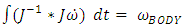
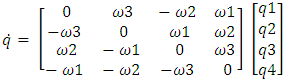
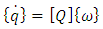
When angular velocity is known, the time invariant solution of the ordinary differential equation in (17), produces a [4x1] dimension quaternion vector (q):

(18)

2.3.3. Direction Cosine Matrix-Quaternion Equivalencies

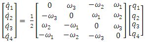
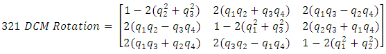
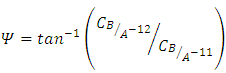
A combined three axis rotation of a rigid body can be expressed with quaternions. The first three elements detail the translation of the three axes, such that the coordinates orient the Euler axis in space. The fourth quaternion details the rotation of the Euler axis about itself. A 3-2-1 rotation can be constructed with quaternions using (19):

(19)

2.3.4. Generation of Euler Angles from Direction Cosine Matrix

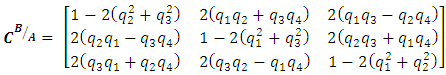
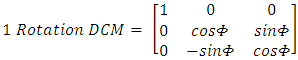
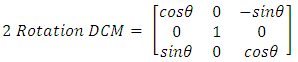
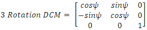
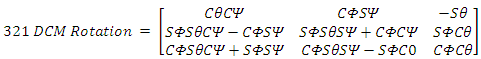
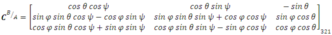
The direction cosine matrix can also be found by the constructing a rotational matrix from the three angles of rotation which normally represent rotational movements of pitch, roll and yaw using component rotations (e.g. equations (7), (8), and (9)).

(20)

The combined sequence of rotations (C^B/A) can be constructed as a single matrix as expressed in equation (10) with the understanding the matrix represents a rotation from basis reference frame A to frame B (e.g. from body to inertial frames) per equation (21).

(21)

By comparing (19) to (19), it is possible to determine the Euler angles for the 3-2-1 rotation sequence per equations (22) through (24) which are equivalent to equations (13) through (15).

(22)

(23)

(24)

2.4. Trajectory Generation

The aforementioned feedforward architectures rely on modeling of dynamic system equations, and furthermore the control equations will be seen to necessitate formulation of a desired full-state trajectory: at least angular velocity and angular acceleration trajectories to formulate the control in addition to angular position to formulate the error.

To accurately model spacecraft maneuvers a standard sine curve (equation (25)) is used to generate a desired trajectory to populate the Trajectory Generator in figure 1.

(25)

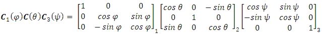
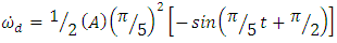
where is the amplitude of the maneuver or the desired angular displacement of the spacecraft. The rate at which the spacecraft completes the maneuver is the frequency of the spacecraft denoted as The phase on the sine curve, used to shift the trajectory curve for smooth onset, is denoted by Using the Commanded Euler Angle and the Desired Slew time in conjunction with equation (25), the commanded maneuver is translated into a trajectory using various sine curves. Equation 25 above is expanded into equations (26) through (28) below for investigations of moment of inertia changes in the dynamics, while equation 26 below is used to investigate and compare numerical methods.

(26)

(27)

(28)

Equations 26-28 feed equation 4, the foundational basis of deterministic artificial intelligence. Using equation (26), the first and second time derivatives provide the commanded angular velocity and acceleration in equations (27) and (28). To ensure system stability, a quiescent time period is provided before the maneuver. The commanded trajectory is implemented over five seconds, after five seconds of quiescent time used to verify correct model operations. The simulation is continued for five seconds after the commanded maneuver to provide sufficient settling time. The Trajectory Generator takes in a commanded body angle and then uses a sine wave in order to approximate the commanded maneuver.

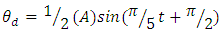
The simulation model’s Trajectory Generator in Figure (1) contains equations 29 through 31 to approximate the commanded maneuver for Angular Position , Angular Velocity and Angular Acceleration via the MATLAB sine wave function.

(29)

(30)

(31)

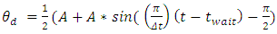
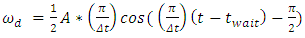
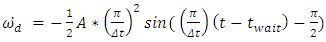
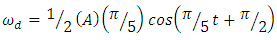
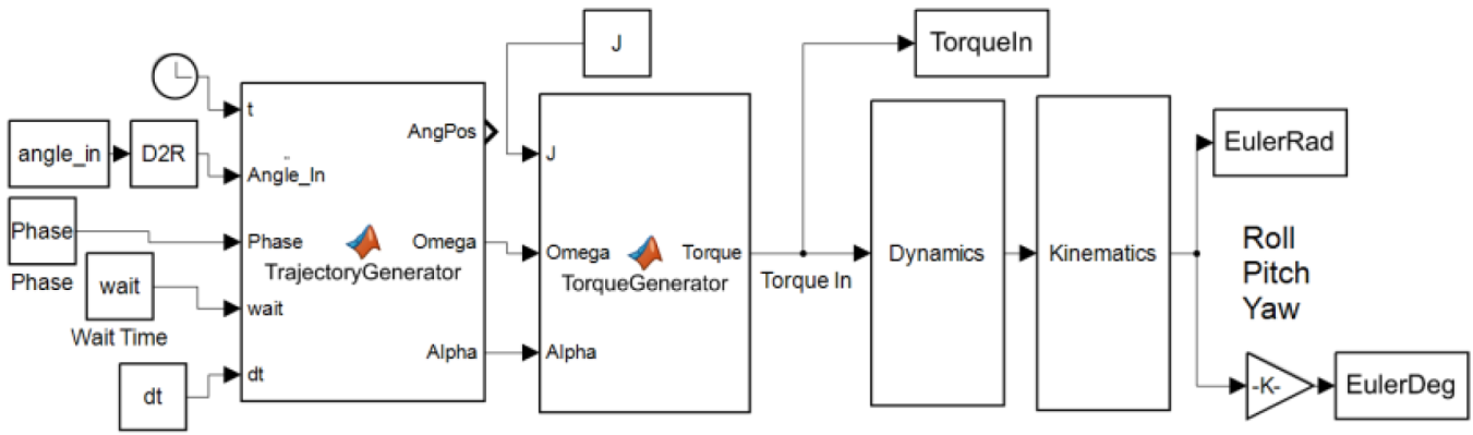
Equation 2-12 models the input command, where A is the maneuver’s commanded angle. The base frequency of the sinusoid is (π/Δt) where (Δt) is the desired maneuver time. The term allows for a quiescent period and -π/2 term allows for a proper phase shift to implement the sinusoidal half period. Equations (30) and (31) are just successive derivatives of equation (29) used to generate angular velocity and acceleration which are fed into the ideal feedforward control equation [46] which resides in the torque generator block of Figure 1. This produces an output torque which drives the dynamics.

2.5. Disturbances

Aerodynamic forces applied over a spatial gradient (stronger at lower altitudes in relatively thicker air) produce an unplanned disturbance torque inducing unplanned rotations. Similarly, Gravity forces are stronger in orbits closer to the center of the earth, resulting in a force gradient generating another disturbance torque producing unplanned rotations. Adaptive and non-adaptive feedforward architectures relying on system identification and disturbance identification [46-59] effectively counter the disturbances and reduce or eliminated the resulting rotational motion. Modeling and analysis are performed in this manuscript for comparison to the efficacy of these methods revealed in the literature.

The ideal feedforward controller must account for the disturbances [25] effecting the spacecraft. Given the relative strength of the gravity gradient and aerodynamic forces in Low Earth Orbit (LEO), the torques from these forces was evaluated for comparison to the ability of fault-tolerant control methods in literature [46-59] to accommodate and reject such.

2.5.1. Aerodynamic Torque

This torque is a result of aerodynamic drag forces acting disparately on the moment arm between the center of gravity and center of pressure on the spacecraft axes of the spacecraft’s body frame (expressed in the Direction Cosine Matrices (direction cosine matrix)) [25]:

(37)

where in equation (37), Ar represents the surface area of the spacecraft in each axis and dL represents the elemental distance from the center of pressure along that axis.

2.5.2. Gravity Gradient Torque

Highly prevalent in low-earth orbits, gravitational torque (resulting from a gravitational force gradient) detailed in equation (38), acts strongly about the y-axis and z- axis (extractable from the direction cosine matrix).

(38)

Gravity gradient torque creates a restoring couple when the spacecraft is displaced from equilibrium, driving the spacecraft back towards its originally stable position. The disturbance torque is accommodated by adjusting the feed forward torque controller to compensate for them:

(39)

3. Results

This section describes the results of each of the major areas of investigation. Dynamics are elaborated with an analysis of the efficacy and impacts of faults resulting in unplanned retention of a spacecraft’s apogee kick motor. Evaluation of computational efficiency [63] produced guidance to researchers about minimum step-size, which was validated in section 3.2.1 of this manuscript. Meanwhile, disturbance environments are analyzed for comparison to the autonomous-rejection capability elaborated in the literature [46-59].

3.1. Dynamics and Changes in Moments of Inertia

To model the effects of a discrete change in moments of inertia, owing to a catastrophic failure as described in section 2.2.1, a Simulink model was used. The Simulink model (topology in Figure 1) consists of five major blocks: Trajectory, Dynamics, Kinematics, Disturbances and direction cosine matrix to Euler Angles. The Trajectory block implements equations (29), (30), and (31) to convert a commanded Euler angle into a desired torque to be fed forward into the Dynamics block. The Dynamics block implements equation (4), converting the inputted torque into an angular velocity in the body frame. The Kinematics lock implements equations (10) - (15), converting angular velocity into quaternions and a direction cosine matrix. The direction cosine matrix to Euler Angles block implements equations (18), (19) and (21) – (24) to convert the direction cosine matrix into Euler angles in the inertial frame. Finally, the disturbances block implements (37) - (38) to determine disturbance torques due to gravity gradient and aerodynamics forces. The Simulink model uses a step size of 0.01s and the ODE4 Runge-Kutta Solver as determined by [63] and validated here in section 3.2.1. For the moment of inertia matrix in (5), a 30° yaw produced the quaternion displacement shown in Figure 4:

Figure 4. Quaternions for the initial nominal [J]

With the loss of the apogee kick motor and the adjustment to a new moment of inertia (6) the quaternions result in Figure 5.

Figure 5. Quaternions for the adjusted [J] post apogee kick motor failure (for various multiples of [J] in equation (6))

Figures 4 and 5 illustrate the impact of the change in moment of inertia, as coupling induces rotation about the other two axes, commencing at the 7.5s mark, after apogee kick motor failure mid-maneuver.

Figure 5 also shows the convergence of the quaternions to erroneous steady-state values as the moment of inertia post-failure is larger than planned in the control. The first two quaternions (proportional to roll and pitch) correctly converge towards zero for the commanded yaw-only maneuver while the third quaternion (proportional to yaw) converges on 0.15 and the fourth quaternion (proportional to the rotation angle) converges on 0.99; illustrating a dampening effect of the moment of inertia via nonlinear coupling as determined by the ratios of mass distributions within the inertia matrix in equation (6).

3.2. Trajectory Generation Computational Investigation

3.2.1. Solver/Integrator Step-size

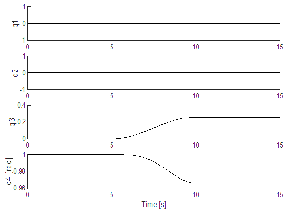
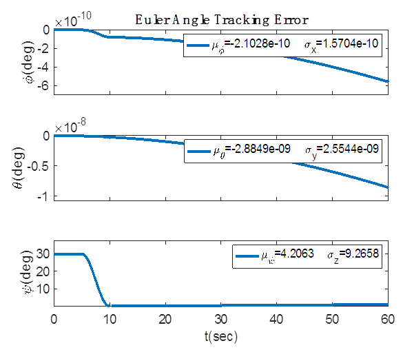
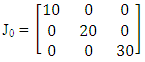
The simulation was run with a fixed step solver using the Runge-Kutta method. In order to determine an appropriate step size for the solver three separate cases were run with three different step sizes. Using 1(blue), 0.1(red) and 0.01(yellow) as examples it became apparent that 0.01 was roughly ideal, as Figure 6 displays correct trajectories for the expected 30 degrees in the Finer iteration followed the previous investigation of computational efficiency.

For the purpose of model verification, commands are initially held constant at zero resulting in zero torque to allow us to evaluate model operation during a quiescent period. With zero input torque, equation (1) shows us that the change in angular momentum should be zero as well; therefore the motion states should not change. After a five second quiescent period, a 30° yaw maneuver was commanded of each model and the maneuver was conducted over a ten second period. Afterwards the output Euler Angles should remain constant with the spacecraft’s new attitude. The results of this test were plotted in Figure 6. Additionally, note that the model was setup with a diagonalized J matrix per equation (5). The roll and pitch Euler Angles remained at zero, as they should have, and as such are not shown.

Figure 6. The Euler angles after a 30 degree yaw, computed using the three step sizes

3.3. Investigation of Disturbances

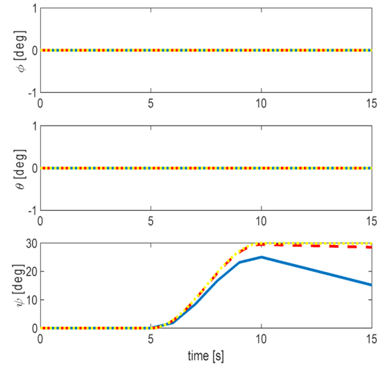
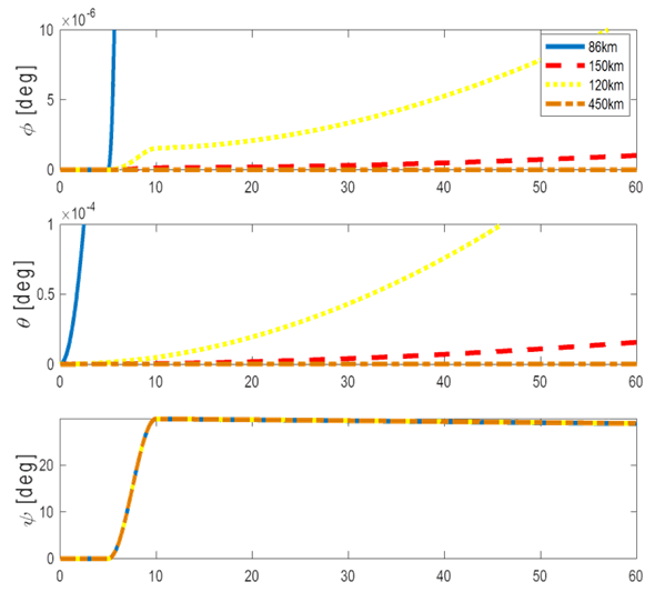
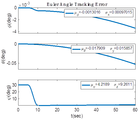
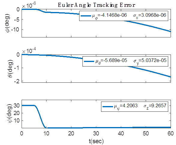
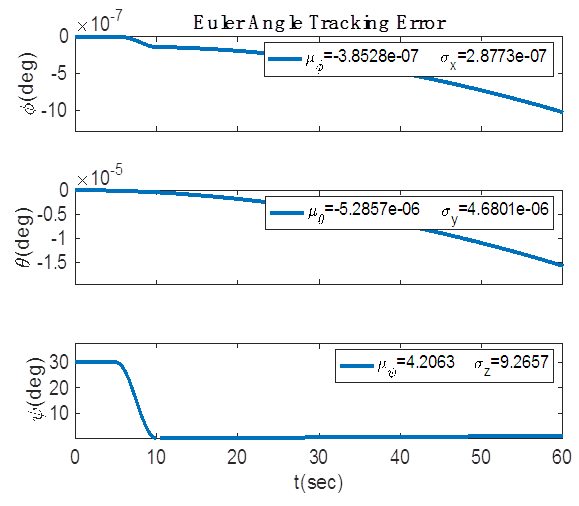
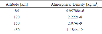
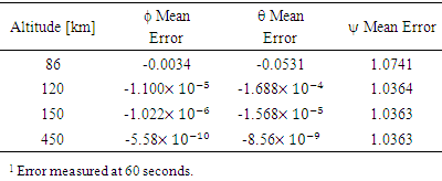
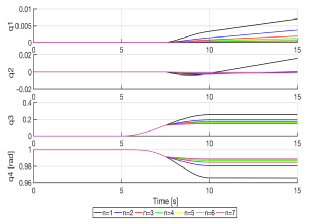
The simulation began with an initial angular velocity of [0 0 0]. Using (3), the angular velocity was input into the kinematics for a maneuver of 30 degrees in the direction. The maneuver is set up to begin 5 seconds into the simulation and take a total of 5 seconds to complete. Figure (7) shows the four separate altitudes corresponding to Table 1 that the aero torque is tested at and the respective atmospheric densities at those heights. Figures 8-11 shows the differing effect of the aero torque on the movement of the spacecraft corresponding to table 2. The maneuver looks increasingly different as the distance from Earth increases as numerically assessed in Table 2. Table 2 shows the numerical decrease in the effect of the aero torque over an increasing distance. In the channel, the error decreases from 0.0034 to 5.58e^-10 over a distance of 364km.

Figure 7. The Euler angles for a 30 degree yaw maneuver. Data represents angles at each of the four different altitudes

Figure 8. Error between input trajectory and Euler angles. 86km

Figure 9. Error between input trajectory and Euler angles. 120km

Figure 10. Error between input trajectory and Euler angles. 150km

Figure 11. Error between input trajectory and Euler angles. 450km

Table 1. Atmospheric densities at four specific altitudes used for calculation of the Aero Torque

Table 2. Euler angles error at the end of the maneuver for each altitude

4. Conclusions

Investigations of unplanned changes in the moment of inertia of space systems revealed resulting motions that were within tolerance of current damage-tolerant algorithms [46-55], [66-67] that rely heavily on these types of modeling efforts to devise intelligent feed-forward control algorithms to anticipate and negate the deleterious effects. The errors are found to favourably compare to the capabilities demonstrated in the recent literature by deterministic artificial intelligence, and this key contribution allows researchers to conclude from this manuscript the strong efficacy in the face of retention of apogee kick motors, even in the presence of realistic orbital disturbances.

Analysis of disturbances confirmed the decreasing effects of the atmosphere with increasing altitudes are predictable, and the assumption that it would decrease significantly was proven. In fact, the decrease was even greater than expected at an even faster rate than expected. It should be noted that the 30 degree maneuver was still completed in the amount of time requested despite the added motion in other dimensions.

Future work should continue the line of research of Nakatani, Cooper, and Heidlauf, but implement their damage-tolerant feedforward methods and the disturbance analysis here to fashion nonlinear feedforward autonomous disturbance-rejection controllers, taking advantage of the computational advice revealed in this study.