1. Introduction

The dynamics of many industrial chemical and biochemical engineering processes can be described by models that take into account transport phenomena (diffusion and convection) and reaction, mathematically translated by partial differential equations (Xu et al., 1993). For example, a tubular reactor or a heat exchanger are characterized by spatial gradients of different temperatures. When the physical system governed by PDEs is translated by evolution phenomena, they take the name of distributed parameter system ([6], [7]).

Several approaches to the synthesis of control laws have been developed for this class of system. According to the methodological approach, the state of the art on command theory shows the existence of two approaches. The first is the discretization of the problem into a set of ordinary differential equations (EDO) using for example the Galerkin or Rayleigh-Ritz methods ([27], [26]). This approach has the advantage to take benefit of the abundant literature offered by finite dimensional synthesis theory [26]. It consists in discretizing the EDP so as to apply the existing finite-dimensional control methods. However, some dynamics of the original system (distributed nature) are lost, it is not easy to prove the convergence of the model properties of the system in finite dimension towards the intrinsic properties of the system in infinite dimension [24].

The difficulties encountered by the equation and solution approximation strategies led the researchers to the idea to develop control strategies based on the direct use of EDP. The methodology consists in the representation of the EDP system in the infinite dimension space during the whole synthesis phase, and the approximation step intervenes only during the simulation. The mathematical tools used in this case are tricky to master and appeal to the theory of functional analysis ([4], [5]). At least they preserve all the information due to the distributed nature of PDEs.

This motivation is due to significant advances in the fields of computer science and instrumentation, thus allowing the scientific community to focus on the use of gradient to describe the quantitative variations of state quantities over time and over space.

In this context, several control laws are developed: [6], [7], [13], [8], [28], [1], [2] and [3].

The majority of these control laws are based on the assumption that the complete state of the system is known. This hypothesis is purely theoretical. In practice, it is rare or even impossible in the case of distributed parameter systems to access to the complete state of the system. Indeed, the dimension of the state space of these systems is infinite, while that of the observations is finite (in other words, the measure is accessible only on certain subsets of the domain of the system). Hence the need to develop software sensors (observers) that can produce an estimation of the variables needed for the synthesis of control laws, and even monitoring, etc.

Distributed models were recently considered in the observation study. Stochastics observers (Kalman filter), that is to say that take into account the noise of measurements and the environment, are presented in infinite dimension in ([21], [28], [32]); set observers based on interval analysis [17] and more recently ([31], [11]). In the deterministic context, Luenberger type observers have been developed by [23], [16], and more recently [12].

In general, classical observers (Luenberger and Kalman) take considerable time to converge, due to the resolution of certain equations (such as the Riccati equation). The choice of setting parameters (the covariance matrices for the Kalman filters) are based on unrealistic assumptions about the nature of the noise.

This paper presents a study on the simulation and observation of a tubular heat exchanger system from a distributed model of the latter.

The novelty of the approach proposed in this manuscript consists in the reconstruction of unmeasured states by using a sliding mode observer ([12], [35]). This observer has several advantages. Beyond its simplicity of tuning, and differently to other observers, it forces the states of the systems to follow perfectly real quantities even in case of disturbances.

The observer's performances are shown through simulations, as part of the temperature estimation of a heat exchanger of the regulatory laboratory of the Polytechnic Faculty of the University of Lubumbashi.

In the next point, we present models of infinite dimension (parabolic and hyperbolic type) of the heat exchanger, and a simulation step follows.

2. Modelling and Simulation of the Heat Exchanger System

2.1. Modelling

The infinite dimensional global mathematical model of the system is described by partial differential equations ([6], [7], [13], [33], [34]). Thermal exchanges between a heat transfer fluid and a porous medium result in diffusion, conduction and convection phenomena.

The heat operator is the main operator with partial derivatives that models the different phenomena (diffusion and convection) within a heat exchanger.

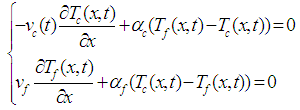
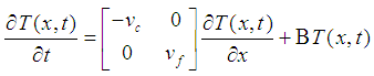
Fluid temperatures are functions of two variables defined on and with values in the real or complex body.

The writing of the energy balance for the inner and outer tube of the heat exchanger respectively leads to the following Diffusion-Convection-Reaction partial differential equations:

(1)

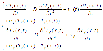
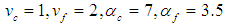
Where and represent the flow velocity of the fluid , the diffusion coefficient and the heat transfer coefficient, respectively. The indices f and c respectively symbolize the cold and the hot.

[6], [7] and recently [13], have explained that diffusion phenomena are frequently neglected () in heat exchangers. This hypothesis reduces the model of the heat exchanger (1) to a Convection-Reaction type model:

(2)

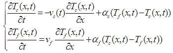
So that the system (2) be completed, it is associated with boundary conditions (Dirichlet or Danckaerts). Which gives for the hot fluid and for the cold fluid (L is length of the exchanger), the boundary conditions of Dirichlet:

(3)

The initial conditions represent the temperature profiles of the hot and the cold fluids under stationary conditions. They are obtained by solving the following system:

(4)

The system (4) is obtained by cancelling the time derivatives in the model of the heat exchanger (2).

It is important to note that the system (4) has two limits. Its resolution has to be considered numerically by means of approximation techniques (finite difference for example).

2.2. Simulation

The lines method [9] leads to the initial profiles of each fluid, represented in the Figure 1, for the set of the following parameters:

•

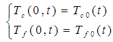
• Boundary conditions for hot fluid

• Boundary conditions for cold fluid

• The number of discretization point ,

• The step of discretization :

Figure 1. Initial temperature profiles of the heat exchanger system

The equations of the system (4) have been integrated by considering a finite difference approximation before each spatial differential operator:

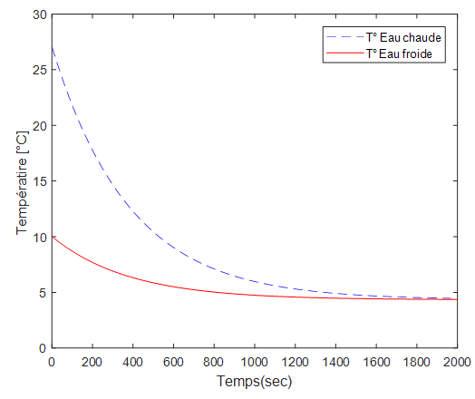
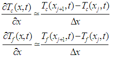The system of ordinary differential equation (EDO) obtained by applying the method of the lines, is solved by using solver ode45 of MATLAB.

Figure 2 shows the spatial-temporal profiles of the temperatures of each fluid in the heat exchanger system.

Figure 2. 3D simulation of heat exchanger temperatures

At the next point we synthesize an SMO for this heat exchanger system.

3. SMO of the Heat Exchanger System in Infinite Dimension

In this section we focus on the design of the SMO in finite dimension for a heat exchanger, in a deterministic context; that is to say where the uncertainties about the measured quantities are not taken into account.

In general, the observability of the systems is studied in the canonical form:

(5)

Following this approach, the heat exchanger system is as follows:

(6)

And the observation equation is:

(7)

The matrix control and observation operators are respectively given by:

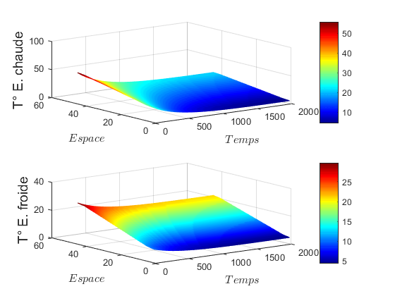
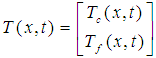Represents the state of the system.

The operator et belong to the Hilbert space defined as follows:

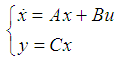
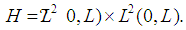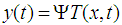
For each , we define a linear application: 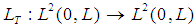, which associates the output y with each input ).

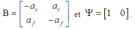
is the space of measurable functions in the real and integrable square body.

In this canonical form of equation, Kalman filters and Luenberger observers were synthesized to estimate unmeasured states [21], [32], [23], [18] and more recently [12]. This literature also shows that the observability of SPD systems is linked to the choice of sensors and their locations.

The originality of our contribution consists into the synthesis of a sliding mode observer ([35], [12]) in infinite dimension. As with any observer, it is based on the model of the system.

Thus for the tubular heat exchanger represented by the EDP system (2), the sliding mode observer is given by the following equation system:

(8)

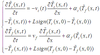
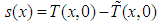Where L is the observation gains matrix, the sign function represents the corrective term and represents the sliding surface.

The term assumes that the state of the system is not measurable everywhere.

4. Presentation of the Results

Figure 3 shows a contra-flow concentric tube heat exchanger from the Control Laboratory of the University of Lubumbashi Polytechnic Faculty.

Figure 3. Heat exchanger

The sliding mode observer (12) will be applied to the datas collected on this system.

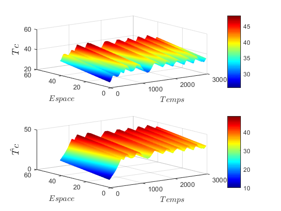
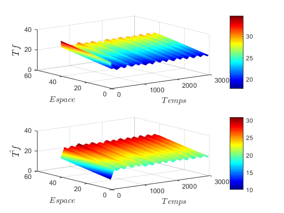
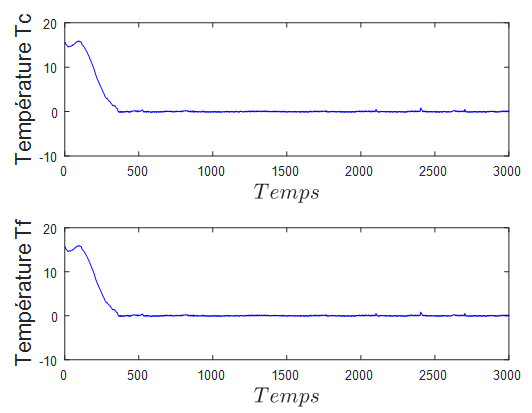
For the simulation, the boundary conditions are taken differently than that of the exchanger, so as to visualize the convergence of the observer. So and .

L is chosen equal to 500. This value is used in a way that its multiplication with the time discretization step is approximately equal to the dynamics of the gaps between successive measured values. The observer was implemented by considering a finite difference approximation before differential operators, with a spatial pitch .

The results of the sliding mode observer for hot and cold fluid are shown in Figure 4.

Figure 4. Evolution of the observation system and the observer for L=500

We can notice in this figure that the dynamics of the system are well estimated, and that the error converges towards zero as shown in Figure 5.

Figure 5. Evolution of the error system for L=500

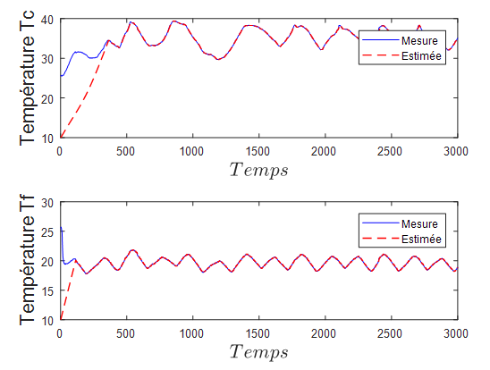
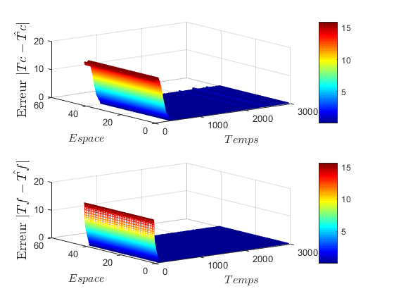
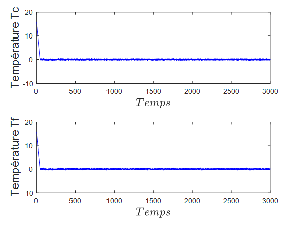
As can be seen, the estimated initial profiles and converge quickly to and respectively, even if they are different at the beginning. This difference is due to the initialization of the boundary conditions of the observer.

To furthermore accelerate the convergence of the observer, we can increase the value of the gain of the latter. With this, the Figure 6 shows the dynamics of the observation system and the observer, for a value of the gain L = 600. It should also be noted in this figure that the increase of the speed of convergence degrades the stability of the observer. In the end, everything is about a compromise speed-stability.

Figure 6. Evolution of the error system for L=600

Figures 7 and 8 show the results of numerical simulation of the observation system and the observer of the hot and cold water temperatures respectively, as a function of time and space. The Matlab ode45 solver was used to dynamically solve the system while taking into account the initial conditions obtained previously.

Figure 7. 3D representation of the observation system and the observer for the hot temperature

Figure 8. 3D representation of the observation system and the observer for the cold temperature

In order to better visualize the dynamics of the observation error system, the evolution of the estimation error of the temperatures at each point of the space considered is presented in the figure (9).

Figure 9. 3D evolution of the error system

5. Conclusions

This article is based on two major problems encountered generally in industrial processes: simulation and estimation of the unmeasured states of the system.

Firstly, we have developed a simulator for a tubular heat exchanger system using the lines method (semi-discretization). The heat exchanger model used here is hyperbolic.

In the second place, an observer was synthesized on this hyperbolic model, in order to estimate the unmeasured states. The originality in this approach comes from the use of a sliding-mode observer in an infinite dimension context of the state space.

The results in simulation have shown the relevance of such approach in the observation of the systems governed by PDEs in a deterministic context.