-
Paper Information
- Paper Submission
-
Journal Information
- About This Journal
- Editorial Board
- Current Issue
- Archive
- Author Guidelines
- Contact Us
International Journal of Control Science and Engineering
p-ISSN: 2168-4952 e-ISSN: 2168-4960
2016; 6(1): 1-11
doi:10.5923/j.control.20160601.01

Trajectory Tracking Control for Six-legged Robot by Correction of Leg Link Target Trajectories Based on LQI Control
 Abstract
 Reference
 Full-Text PDF
 Full-text HTML
Hiroaki Uchida
Department of Mechanical Engineering, National Institute of Technology, Kisarazu College, Kisarazu, Japan
Correspondence to: Hiroaki Uchida, Department of Mechanical Engineering, National Institute of Technology, Kisarazu College, Kisarazu, Japan.
| Email: |  |
Copyright © 2016 Scientific & Academic Publishing. All Rights Reserved.
This work is licensed under the Creative Commons Attribution International License (CC BY).
http://creativecommons.org/licenses/by/4.0/

In this study, a trajectory tracking control method for the walking direction of a six-legged robot was developed. We proposed an error correction method for the motion of the rotating links in the horizontal direction and the yaw angle. From the proposed control method, the equations of motion in the x and y directions and the yaw angle of the robot’s motion were derived, and an optimal linear-quadratic-integral (LQI) servo system was introduced. The walking directional control inputs were converted to modified signals for the rotation angles in the support phase. The modified signals were then added to the reference signals for the original trajectory. A proportional-derivative controller for each rotating link in the support phase received the modified signal. The LQI controller worked to decrease the errors between the planned trajectory and the actual trajectory. We examined the effectiveness of the proposed control design method using 3D simulations of a robot following straight and semicircular trajectories.
Keywords: Six-legged Robot, Walking Directional Control, Trajectory Tracking Control, LQI Control, 3D Simulation
Cite this paper: Hiroaki Uchida, Trajectory Tracking Control for Six-legged Robot by Correction of Leg Link Target Trajectories Based on LQI Control, International Journal of Control Science and Engineering, Vol. 6 No. 1, 2016, pp. 1-11. doi: 10.5923/j.control.20160601.01.
Article Outline
1. Introduction
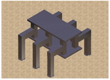
- Multi-legged robots can operate under extreme conditions where it is difficult for humans to work, and a wide variety of research has been carried out on topics relating to four- and six-legged robots, including mechanisms [1, 2], control methods [3], control systems [4], gait/walking planning [5-11], and energy consumption [12]. Hirose et. al. [5] examined the relationship between the supporting legs and the position of the robot's center of gravity that would allow a four-legged robot to walk in a circular path. In the walking simulations/experiments in these studies, leg joints are modeled as if they are following a planned trajectory, and the influence of tracking errors is rarely considered. Recently, the popularization of global position satellite systems, laser rangefinders (LRFs), and stereo cameras has made possible the autonomous recognition of walking environments [13] and the measurement and estimation of position for localization systems [14] by multi-legged robots. Cobano et al. [15] investigated a method of target trajectory tracking based on self-position estimation [14]. Go et al. [16] conducted local feedback (FB) control that tracks the target angle of leg links by measuring the deviation from the target trajectory and then correcting the target trajectory. This method requires constant correction of the target trajectory while walking. Also, when walking on uneven terrain, the height between the supporting legs and the walking surface will differ for each leg, and there is no guarantee that the target values for each leg link, which are calculated beforehand based on the walking plan, will conform to the planned trajectory during operation. Therefore, in terms of the walking direction, three degrees of freedom-body position (x, y) and posture angle (yaw angle) in regard to the walking surface-must be controlled using FB control so that they follow the target trajectory. Also, the three degrees of freedom of body height, pitch angle, and roll angle must be controlled in order to achieve a stable posture on uneven terrain. In terms of posture control, there are studies that examined the subject from the perspective of control methods that consider robot dynamics [17, 18]. In one such study [18], the authors used a six-legged robot with a leg mechanism proposed by Hirose et al. [19] to investigate a posture control method. The body height, pitch angle, and roll angle were controlled by the thigh link (Fig.1) during walking with three-legged support, and a 3D simulation was used to demonstrate the method's effectiveness. However, as far as we are aware, very little research has been done on methods for FB control of the walking direction (x, y and yaw angle) from the perspective of control system design. This study investigates a method for simultaneously controlling the body position (x, y) and yaw angle for a six-legged robot using the above-mentioned leg mechanism. The leg mechanism has three degrees of freedom, which are a rotating link, a thigh link, and a shank link. In terms of controlling the walking direction of the body, omnidirectional walking is achievable by controlling the rotating link and the shank link. This study examines walking directional control using the rotating link only, in order to simplify the problem. Specifically, when walking with three-legged support, the reaction force from the rotating link becomes a propulsive force in the body, and so we derive a mathematical model for controlling the body position (x, y) and yaw angle in this situation. For this model, we build a type-1 servo system and design a linear-quadratic-integral (LQI) control system so that the robot follows the target trajectories of body position (x, y) and yaw angle. The FB inputs acquired by the LQI control system are converted into correction amounts for the target angles of the rotating link of the supporting legs, and the target trajectories of the rotating links are corrected. The effectiveness of the proposed method is confirmed by simulation using a 3D model of the six-legged robot.
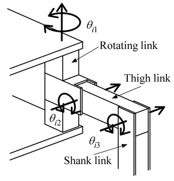 | Figure 1. Model of robot leg |
2. Six-legged Robot and 3D CAD Model
- Figure 2 shows the six-legged robot used in this study, and Table 1 shows its specifications. Figure 1 shows a model of one of the legs. Each leg has three degrees of freedom, which are a rotating link, a thigh link, and a shank link, and the leg mechanism is such that the velocity of the robot's body is generated by the rotating link, while the weight of the body is supported by the thigh link. Also, the shank is capable of moving in directions in which it is difficult for the rotating link to move, but this study does not examine the capabilities of the shank. Each leg link is driven by a worm gear. The self-locking function of the worm gear cancels torque due to body weight in the thigh link. The motion of the robot is driven by the control input, which requires a current flowing from the motor driver to the motor through a D/A converter. The body of the robot is equipped with a LRF, a posture sensor that detects the body's pitch angle and roll angle, and an ultrasonic sensor that detects the height of the body. Figure 3 shows a 3D CAD model of the six-legged robot shown in Fig. 1. The model was created by connecting a total of 19 elements (1 body, 3 leg joints) using revolute joints. An experiment on the frequency response was conducted using a leg joint of the six-legged robot. Each revolute joint is approximated using the following second-order transfer function.
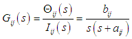 | (1) |
|
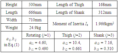
 | Figure 2. Six-legged robot |
 | Figure 3. 3D CAD model of six-legged robot |
 represents the leg link rotation angle,
  represents the command current to the motor driver, i represents leg number (1 to 6), and j represents the rotating link (1), the thigh link (2), or the shank link (3). Table 1 shows the
  and
and  values for the rotating link, thigh link, and shank link. Also, four contact points are present on the underside of the foot at the end of each leg, and contact with the walking surface is modeled using springs
  and dampers
  , and the coefficient of friction is taken to be 0.35. In this study, the robot is modeled in 3D using Virtual.Lab Motion, and numerical calculations are done using MATLAB/Simulink. Nonlinear equation of motion for the robot is derived automatically in Virtual. Lab Motion. Also, the mechanism in the actual robot is such that the shank and the underside of the foot are connected by a revolute joint, and the entire underside of the foot makes contact with the walking surface. However, this revolute joint is not included in the 3D CAD model. The influence of the error caused by the absence of this revolute joint in the model is reduced by designing the walking trajectory as follows: (1) The trajectory is such that the shank is always roughly perpendicular to the walking surface. (2) The walking speed is such that the influence of slippage of a supporting leg in the 3D simulation is small. This assumes stable operation / walking on uneven terrain. In the simulation, the maximum slip velocity in the x and y directions is 0.002 m/s, and approximately 0.01 m of slippage occurs in a 5-second support phase. The control method in this study is affected by the reaction forces acting on the supporting legs, and so it is preferable that there is no slippage. However, it is impossible to create a walking environment in which there is absolutely no slippage, and so the effectiveness of the control method is tested in a walking environment where this slippage occurs in the supporting legs.
3. Walking Plan and Walking Trajectory Design
- When the robot is made to walk along a target trajectory in a walking space, it is necessary to control the position of the center of gravity and the yaw angle of the body in the support phase. This requires consideration of the gait pattern, the trajectories of the supporting and swinging legs, FB control of the center of gravity and the posture in the support phase. This study focuses on designing a system for FB control of the center of gravity and the posture. Therefore, the gait pattern was taken to be the pattern of Wave Gait with duty factor of 50% [20] shown in Fig. 4, which can be controlled by the FB control system. Also, to simplify the problem, in this study a system is designed for controlling the body's center of gravity using the rotating link only. In this case, for the robot used in this study, a large value can be taken for the displacement of the rotating link of the supporting legs in the direction of movement
 (the distance traveled by the robot), but a large value cannot be taken for the displacement perpendicular to the direction of travel
  because the supporting leg's rotating link approaches a singularity. A typical approach is to design target trajectories for the body's center of gravity and the tip of each leg, convert these into target trajectories for the leg links using inverse kinematics [21], and then control the robot's legs by local FB control of each leg link. In this situation, the body's center of gravity does not follow the target trajectory due to factors such as tracking errors resulting from local FB, and slippage of the ends of the supporting legs. Therefore, a trajectory tracking control system is designed that minimizes the deviation by constantly updating the body's center of gravity and posture
  The coordinates of the three supporting legs have a large influence in this FB control system, and so the design of the swing leg trajectories is important. Typically, the walking trajectory of a multi-legged robot can be constructed by combining straight-ahead and turning trajectories.
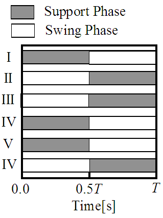 | Figure 4. Walking patterns |
3.1. Trajectory of Robot's Center of Gravity While Turning
- Figure 5 shows the relationship between the axis of rotation, the coordinates of the center of gravity, and the supporting leg positions when the robot moves in a circle with three-legged support. The simulated trajectory of the robot's center of gravity is taken to be the position of the robot body's center of gravity
 making a circular motion with a radius
  around the axis of rotation
  The orientation of the robot's body is assumed to remain tangential to the circular path. The height of the robot's center of gravity
  is assumed to be constant, and the pitch and roll angles are assumed to be rad. The trajectory of the robot's center of gravity in the global coordinate system is given by Eq. (2). The origin of the global coordinate system is taken to be the initial position of the robot. The direction of travel of the robot is taken to be along the
  -axis, and the horizontal direction perpendicular to the -axis is taken as the
 | (2) |
3.2. Trajectory of Ends of Legs While Turning
- The robot walks with a tripod gait, which means that Legs I, IV, and V and Legs II, III, and VI alternate repeatedly between a support phase and a swing phase. In Fig. 5, it is assumed that in one walking cycle the robot's center of gravity advances by an angle of
 on a circular path of radius
  around the axis of rotation
  The distance travelled by Leg VI before and after the walking cycle in the -axis and -axis directions is taken to be
  and
and  respectively. The trajectory of the end of the leg during the swing phase of one walking cycle is assumed to be a linear interpolation of this distance. The trajectories of Legs I–V are also designed using the same method. The trajectories obtained using the global coordinate system are converted to the robot coordinate system using a rotation matrix, and then transformed into target trajectories for leg joint angles using inverse kinematics.
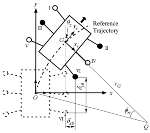 | Figure 5. Relation between center of gravity and center of rotation for six-legged robot during circular walk |
4. Walking Directional Control Method
4.1. Converting from Global Coordinate System to Robot Coordinate System
- The robot’s trajectory is described in the global coordinate space, and so it is necessary to convert the target trajectories into the robot coordinate system. The origin of the robot coordinate system is the center of gravity of the robot's body. Figure 6 shows the error relative to the target trajectory in the robot coordinate system.
 represent the error in the center of gravity in the
  directions in the robot coordinate system.
  represents the angle of the direction of travel (yaw angle) for the robot in the global coordinate system.
  are obtained by converting the error in the global coordinate system into the robot coordinate system using the rotation matrix.
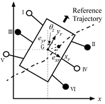 | Figure 6. Relation between robot’s local coordinate system and global coordinate system |
4.2. Mathematical Model for Six-legged Robot
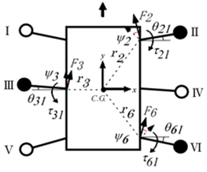
- Figure 7 shows the relationship between the torque generated by the rotating link with three-legged support and the force working to the body by this reaction force. In the figure, the supporting legs are Legs II, III, and VI; while the swinging legs are Legs I, IV, and V. Also, it is assumed that the supporting legs land firmly on the walking surface and no slippage occurs at the points of contact. Here,
 represents the direction of travel in the robot coordinate system,
  represents the horizontal direction perpendicular to the
  -axis, and
  represents the yaw angle of the robot's body, which is the angle of rotation about the
  In Fig. 7,
  is taken to be the reaction force received by the body's revolute joint from the supporting leg,
  represents the body's mass,
  is the moment of inertia about the
  and
and  is the angle of the revolute joint in the rotating link. For
 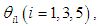 the clockwise direction is taken as positive, while for
 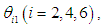 the counterclockwise direction is taken as positive.
  represents the position vector from the center of gravity of the robot's body to the rotational center of the rotating link of each leg. Figure 8 shows the relationship between the force
  acting on supporting leg II, and the force
  which is the component of
  that acts perpendicular to
  . indicates the angle between
  and
and  The equations of motion for the center of gravity of the robot's body in the
  direction,
  direction, and about the yaw angle
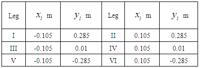
  are shown below. The equations of motion are derived in the same way for the situation where Legs I, IV, and V are supporting legs. Table 2 shows the
  and
and  coordinates of the rotational center of the rotating link of Legs I–VI.
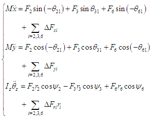 | (3) |
|
 | Figure 7. Forces acting on three supporting legs |
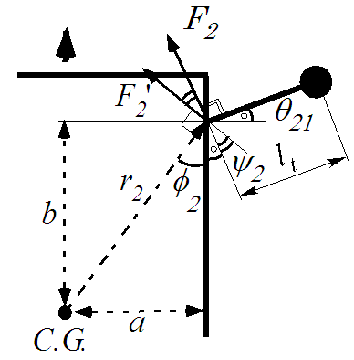 | Figure 8. Relation among  |
 The forces
  and
and  represent the components of
  in the
  and
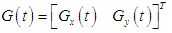
and  directions and in a circumferential direction about the body's center of gravity, and they are treated as disturbances. In this study, the effect of the slippage is large as the disturbance in Eq.(3). In real walking of the robot, the disturbance depends on the walking surface. The proposed control method can deal with the variation of the reaction force from the walking surface.Defining the state variable vector as
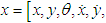
 and the control input vector as
 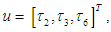 gives the following state and output equations:
 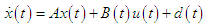 | (4-a) |
 | (4-b) |
 is a time-varying matrix.
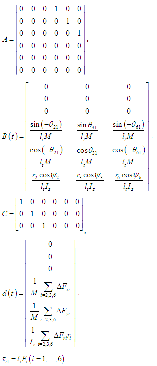
4.3. Optimal Servo System
- Taking the target vector to be
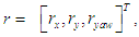 a type-1 servo system is designed for a mechanism which is affected by the disturbance expressed in Equation (4). The steady state is the situation in which each leg link is controlled by a PD control system to follow the target trajectory of each leg joint, calculated using inverse kinematics from the walking trajectory presented in Section 3. The main sources of errors between the controlled variables and the target trajectory are the disturbance
  expressed by Equation (4-a) and the tracking performance of the PD control system. This disturbance is treated as a step disturbance. A type-1 servo system is effective for reducing step disturbances.
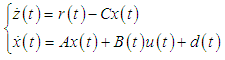 | (5) |
 | (6) |
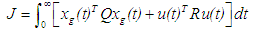 | (7) |
 and
and  are weighting matrices given by the design specifications, where
  The control input
  used to minimize Eq. (7) is given by the following equation:
 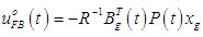 | (8) |
 is the unique positive definite solution of the following Riccati equation:
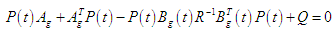 | (9) |
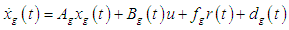
4.4. Time-invariant Optimal Servo System
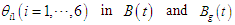
- The FB system described in Section 4.3 is a time-varying system, and when it is used to control the robot, Eq. (9) has to be solved at every sampling time, which is a burden on the controller. Therefore, to make the FB equation time invariant, the input matrix
 for the system given by Eq. (5) is fixed at a certain angle
 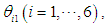 in the range of movement of each rotating link. The range of movement of each rotating link is given by the following equations:
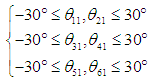 | (10) |
 given in Eqs. (5), (6), (8), and (9) are fixed as follows.
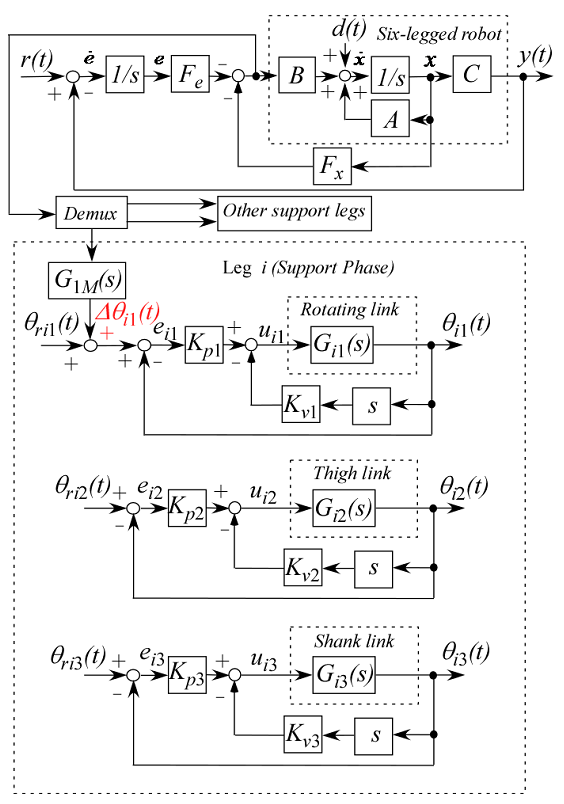
  are set to 15°. When
  are positive,
  and when
 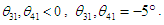 And
And 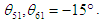
4.5. Method for Correcting Target Trajectory of Supporting Leg Rotating Link
- Figure 9 shows a block diagram illustrating walking directional control and control of each leg link in one supporting leg. The PD control for each leg link in Fig. 9 is given by the following equation:
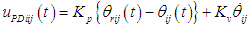 | (11) |
 | Figure 9. Block diagram of walking directional control for one support leg |
 indicates the proportional gain, and
  is the velocity gain.If the PD control input
  that tracks the target trajectory and the FB control input
  obtained from Eq. (8) for walking directional control, are added together and inputted, the FB control input becomes excessive, and may cause damage to the motor driver or the motor in the robot. And, there are non-linear characteristics of the saturation and the dead-zone in the motor. Therefore, the FB control input obtained from Eq. (8) is converted into an angle that corrects the target trajectory of the supporting leg's rotating link. The correction method determines the size of the angle correction
  using the transfer function given in Eq. (1), and corrects
  in Eq. (11).
5. 3D Simulations
- The simulation is conducted in MATLAB/Simulink for two cases, Case I, where the robot walks in a straight line, and Case II, where it walks in a semicircle. The weighting matrices in Eq.(7) are determined by the trial-and-error method.In Case I, 10 walking cycles are performed, with each step being 0.12 m and one period T=10 s. The target values for the center of gravity of the robot body
 and the yaw angle are set to zero, and the target trajectory in the direction of travel
 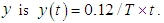 Consequently, all leg joints are controlled by the PD control input
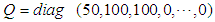
  to follow the target trajectory. The weighting matrices in Eq. (7) are
  and
and  Figures 10–12 show the results of the 3D simulations. Figures 10(a)–(c) show the time response waveform for the robot's center of gravity
  and the yaw angle, respectively. When each leg link follows the target trajectory using only PD control, the error increases with respect to the target trajectory in the
  direction of travel. The error with respect to the target value after 10 walking cycles is 0.22 m, or 18.4%. This is because slippage occurs on the underside of the foot of the supporting legs, and the slippage accumulates as the number of walking cycles increases. However, using combined PD and FB control (walking directional control) proposed in this study, the error decreases to 0.03 m, or 2.6%. This is because the FB control performs an error correction. These results confirm the effectiveness of the proposed method. In the
  direction, deviation occurs for both PD control only and combined PD and FB control. This is because the weighting for the
  values when FB control is added is smaller than the weighting for the
  and yaw angle values. Also, in the robot's mechanism, the rotating link approaches a singularity in the
  -direction, and so control performance is inferior to that for the
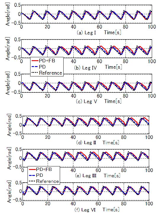
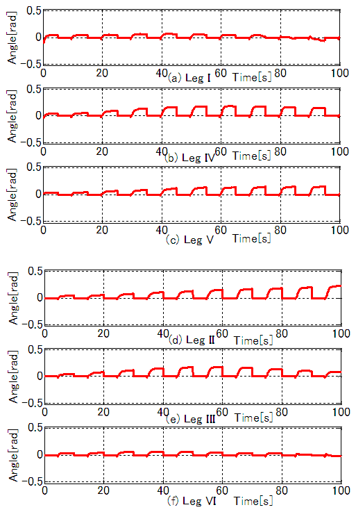
  -axis and yaw angle. With regard to the yaw angle, the addition of FB control causes vibration, but its amplitude is small at 0.03 rad. Figure 11 shows the time response waveform for the rotating link of each leg. Figures 11(a)–(c) show the results for Legs I, IV, and V; and Figs. 11(d)–(f) show the results for Legs II, III, and VI. The solid red line indicates PD + FB control, the blue dashed line indicates PD control only, and the black dotted line indicates the target trajectory. Figure 12 shows the time response waveform for the angle correction in the rotating link of the supporting legs obtained by FB control input. It can be seen that a positive correction angle is used for each supporting leg. This is because, for PD control only, slippage of the ends of the legs causes the trajectory of the robot's center of gravity to advance ahead of the target trajectory, and the center of gravity is controlled by correcting the target trajectories of the rotating links. As a result, the center of gravity and yaw angle for the robot's body are controlled to follow the target trajectory.
 | Figure 10. Simulation results for position and yaw angle (straight trajectory) |
 | Figure 11. Simulation results of rotating angles (straight trajectory) |
 | Figure 12. Simulation results for correction angles obtained by FB inputs (straight trajectory) |
 and
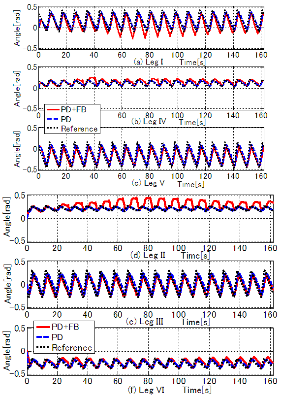
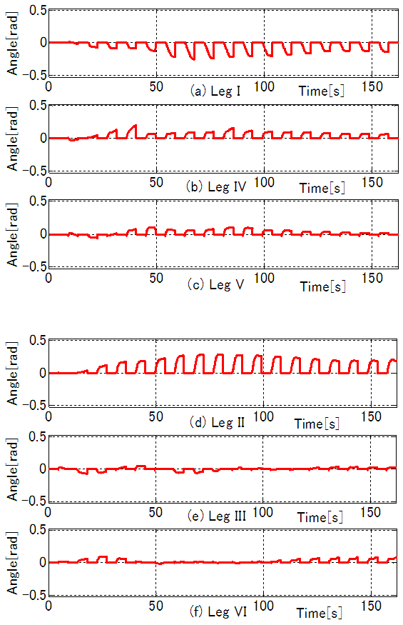
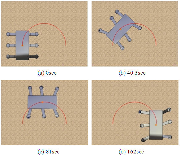
and 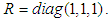 The results in Figures 13(a)–(d) show that using combined PD and FB control, x, y, and the yaw angle are controlled to follow the target trajectory. In the simulation, using only PD control, it is evident that errors accumulate due to factors such as tracking errors and slippage at the ends of the supporting legs. For combined PD and FB control, the position of the body's center of gravity is steered to follow the target trajectory. The -axis in Fig. 13(b) shows a tracking error at the end point of 0.00 m (0.35%) with combined PD and FB control, compared to 0.38 m (38%) with PD control. The yaw angle in Fig. 13(c) shows a tracking error at the end point of -0.026 rad (1.00%) with combined PD and FB control, compared to -0.680 rad (21.7%) with PD control. These results show an improvement in the tracking performance with combined PD and FB control. Figure 14 shows the time response waveform of the rotating link of each leg. The solid red line indicates combined PD and FB control, the blue dashed line indicates PD control only, and the black dotted line indicates the target trajectory. Figure 15 shows the time response waveform of the angle correction in the rotating link of the supporting legs obtained by FB control inputs. For combined PD and FB control, the size of the target angle correction for Legs I and II during the support phase is larger than for the other legs, and it is evident that deviation from the target trajectory is corrected by correcting the target angle of the front supporting leg in three-legged support. Figure 16 shows the animation results in Case II. Figure 16(a) shows the initial position and posture at t = 0 s, Figs. 16(b) and 16(c) show the positions at t = 40.5 and 81 s, respectively, and Fig. 16(d) shows the position and posture at the end point. The solid red line indicates the target trajectory in the x-y plane. These results show that the method proposed in this study is effective for trajectory tracking control of the robot.
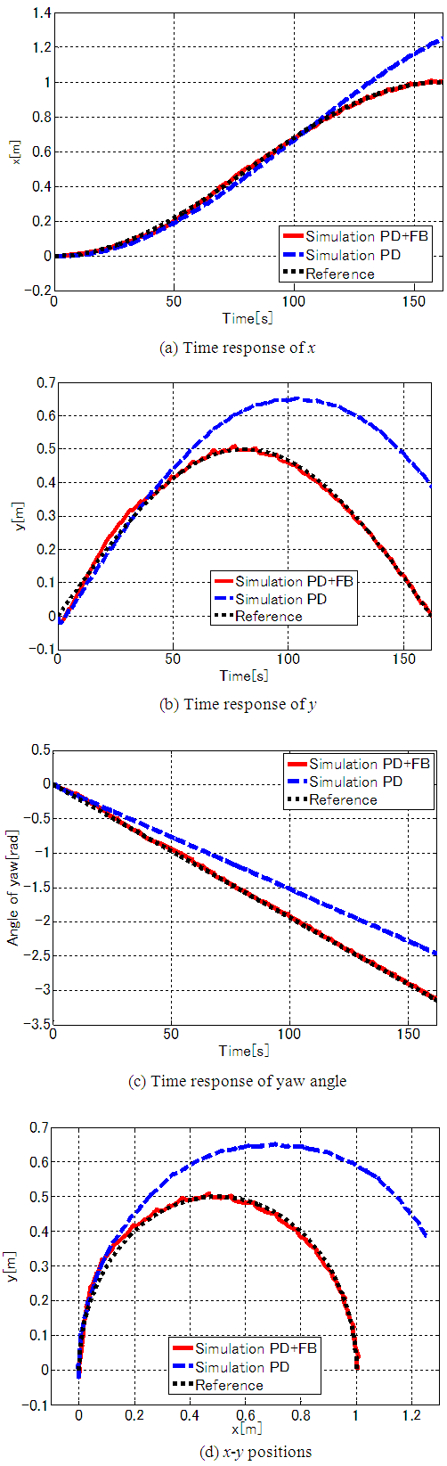 | Figure 13. Simulation results for position and yaw angle (semicircular trajectory) |
 | Figure 14. Simulation results for rotation angles (semicircular trajectory) |
 | Figure 15. Simulation results for correction angles obtained by FB inputs (semicircular trajectory) |
 | Figure 16. Animations of semi-circle walking trajectory |
6. Conclusions
- This study investigated a method of trajectory tracking control for a six-legged robot in a walking environment, whereby the center of gravity of the robot's body (x, y) and posture angle (yaw angle) follow target trajectories. The following results were obtained:1. A mathematical model was derived for the robot’s trajectory when its body is propelled by reaction forces acting on the supporting legs. FB control using an optimal servo system was designed to perform a corrective operation to reduce errors between the target trajectory and the center of gravity of the robot's body (x, y) and posture angle (yaw angle), so that the robot follows the target trajectory.2. The effectiveness of the proposed FB control system was validated in a 3D simulation of the robot. Trajectory tracking control was performed for straight and semicircular target trajectories with and without the FB control system. When the FB control system was not used, errors between the actual and target trajectory increased as a result of factors such as slippage of the supporting legs. However, when FB control was added, corrective action to reduce errors was taken, and the robot followed the target trajectory. In this case, the FB inputs acquired by the LQI control system were converted into correction amounts for the target angles of the rotating link of the supporting legs, and added to the target leg link angles obtained from the trajectory plan. The rotating link was controlled with the PD control method to follow the corrected target trajectory.
ACKNOWLEDGEMENTS
- Walking simulations of this research were done with cooperation of Noriyuki Shiina in National Institute of Technology, Kisarazu College (those days). This work was supported by JSPS KAKENHI Grant Numbers 25420200.