1. Introduction

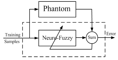
Robotics is a new branch of science that encompasses several areas such as industry, medicine, aerospace, etc. [1]. Robot control and its practical simulation require an accurate, yet simple dynamic model [2]. An important task of a control engineer in designing and developing a control procedure is to develop a mathematical model that describes the actual robot behaviour. The actual robot model may be too complicated and its dynamics may not be totally understood. Developing a mathematical model that can accurately describe the physical behaviour of the robot over an operating range is a challenging task. Even if a detailed mathematical model of the robot is available, such a model may be of high order leading to a complex controller whose implementation may be costly and whose operation may not be well understood. Generally, there are two basic methods to obtain the models of the systems. The first method is based on the physical laws governing a particular system and the second method involves modeling a system using system identification methods [3]. System identification deals with the selection of the mathematical models to describe the input–output behaviour of an unknown system by means of data obtained from the process. Linear system identification developed significantly in the past decades. However, these methods could not accurately describe complex non–linear systems [4-5].

Since most industrial processes display non–linear and time–varying behaviours, linear mathematical models cannot demonstrate the behaviour of the system over its full operational range. Accordingly, there has been a growing research interest in non–linear identification of models. Non–linear identification techniques such as bilinear models [6], Wiener–Hammerstein block–oriented models [7], Non–linear Auto Regressive Moving Average eXogenous (NARMAX) models [8], and fuzzy models [9], have been proposed to solve this problem.

Artificial Neural Networks (ANNs) have been widely used to model unknown systems. It has been demonstrated that an ANN can approximate a wide range of non–linear functions to any desired degree of accuracy under certain conditions. Based on its capability, it is not necessary to spend much effort on system modeling, while developing a mathematical model that describes accurately the physical behaviour of the unknown system over an operating range is a challenging problem [10].

Fuzzy logic systems (FLS) have gained vast development in modeling complex non–linear plants. Since FLS are constructed from fuzzy IF–THEN rules, the details of the mathematical model are not required. Moreover, FLS can express adequately non–linearities and uncertainties in systems, which cannot be described by precise mathematical models. According to the universal approximation theorem [11, 12], any non–linear function over a compact set can be approximated by FLS with arbitrary accuracy [13].

Recently, neuro–fuzzy computing approach has been developed as a consequence of combining both these methods, i.e., ANN and FLS. Adaptive Neural network based Fuzzy Inference System (ANFIS) was proposed by Jang [14] combines the neural network adaptive capabilities and the fuzzy logic qualitative approach. Therefore, ANFIS has both benefits of ANN model, i.e., computational power and FLS model, i.e., human like thinking. ANFIS has reached its popularity due to a broad range of useful applications in such diverse areas in recent years as optimization of fishing predictions [15], vehicular navigation [16], identify the turbine speed dynamics [17], radio frequency power amplifier linearization [18], microwave application [19], image de–noising [20, 21], prediction in cleaning with high pressure water [22], sensor calibration [23], fetal electrocardiogram extraction from ECG signal captured from mother [24], identification of normal and glaucomatous eyes [25].

These applications show that ANFIS is a good universal approximation method, predictor, interpolator, and estimator. They demonstrate that each non–linear function of many inputs and outputs can be easily constructed with ANFIS. An important task of a control engineer in designing and developing a control procedure is to obtain a mathematical model that describes the actual plant. The actual plant may be too complicated and also its dynamics may not be totally understood. Developing a mathematical model that describes accurately the physical behaviour of the plant over an operating range is a challenging task. Even if a detailed mathematical model of the plant is available, such a model may be of high order leading to a complex controller whose implementation may be costly and whose operation may not be well understood. Dynamic behaviour of ANFIS motivates us in this study to use it in non–linear modelling of a Phantom robot. Moreover, five different methods are implemented for comparison with the proposed method. These approaches are Artificial Neural Networks (ANNs) with Gradient Descent with Momentum Back Propagation (GDM BP), Gradient Descent with Adaptive learning rule Back Propagation (GDA BP), Levenberg–Marquardt Back Propagation (LM BP), Radial Bias Function network (RBF), and Least Square Support Vector Regression (LS–SVR). Three error measurement indices are used to verify the validation of the proposed method in comparison with the other methods.

The rest of this paper is organized as follows. In Section 2 the problem statement is defined. Then, in Section 3 the ANFIS architecture formulation is briefly reviewed. Experimental results and discussions on the Phantom robot are performed and compared with other identification method in the literature to support accuracy of the ANFIS model in section 4. Finally, Conclusions are drawn in Section 5.

2. Problem Statement

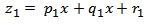
Phantom robot is a desktop device developed by SensAble Technologies, Inc. with three degrees–of–freedom (DOF). This robot has been widely used in tele-robotic applications [26]. The schematic diagram of the device with three motors and the corresponding joint angles, θ₁, θ₂, and θ₃ is shown in Figure 1.

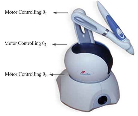Figure 1. Phantom robot

The functionality of the robot is affected by its unknown electrical and software sub systems. To achieve accurate control and simulation of the device, precise dynamic models of the robot are needed. The dynamics of a robotic joint can be formulated as shown in (1):

(1)

where M, C, and N represent the inertial matrix, Coriolis and centrifugal matrix, and gravitational vector respectively, defined in terms of the inertial and kinematic properties of the robot individual components [27]. Here, and are respectively torques vector delivered by the motors and the vector of joint angles derived from the encoders [28, 29]. Although it is feasible to calculate a mathematical model for the robot based on physical rules, the complexity of the obtained model imposes some difficulties on practical implementation. ANFIS as an identification method taken away from the complexity of the model of Phantom robot and its physical rules.

3. Adaptive Neuro–Fuzzy Inference System (ANFIS) Architecture

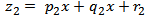
Non–linear function of many inputs and outputs can be easily constructed with the ANFIS model. A typical architecture of the model is illustrated in Figure 2, in which a circle indicates a fixed node and a square depicts an adaptive node. For simplicity, two inputs i.e., x and y, and one output i.e., z, in the fuzzy inference system (FIS) can be considered. The ANFIS implements a Sugeno–Fuzzy type inference system. For example, for a Sugeno–Fuzzy model, a common rule set with two fuzzy if–then rules can be expressed as follows:

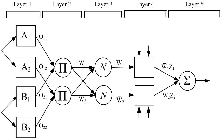Figure 2. ANFIS architecture are defined in (6), (7), (9), respectively

Rule 1: If x is A₁ and y is B₁,

Then

(2)

Rule 2: If x is A2 and y is B₂,

Then

(3)

where and are fuzzy sets in the antecedent, and are the design parameters that are determined during the training process.

As shown in Figure 2, the ANFIS consists of five layers: Layer 1, every node in this layer is an adaptive node with a node function:

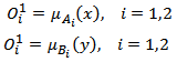(4)

where x, y are the input of node and and can adopt any fuzzy Membership Function (MF). In this paper, Gaussian MFs are used:

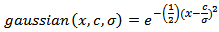(5)

where is center of Gaussian MF and is a standard deviation of this cluster. In layer 2, every node represents the ring strength of a rule by multiplying the incoming signals and forwarding the product as:

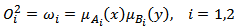(6)

In layer 3, the i–th node calculates the ratio of the i–th rules ring strength to the sum of all rules ring strengths:

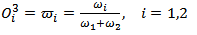(7)

where is referred to as the normalized ring strengths. In layer 4, the node function is represented by

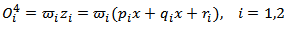(8)

where is the output of layer 3, and are the parameter set which are referred to as the consequent parameters.

In layer 5, the single node computes the overall output as the summation of all incoming signals:

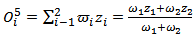(9)

It is clear that the ANFIS has two sets of adjustable parameters, namely the premise and consequent parameters. During the learning process, the premise parameters in the first layer and the consequent parameters in the fourth layer are tuned until the desired response of the FIS is achieved. In this work, an Adaptive Neuro–Fuzzy Inference System (ANFIS) model is utilized to rapidly train and adapt the FIS. When the premise parameter values of the membership function are fixed, the output of the ANFIS can be written as a linear combination of the consequent parameters:

(10)

The LS method can be applied to determine optimally the values of the consequent parameters. When the premise parameters are not fixed, the search space becomes larger and the convergence of training becomes slower. The hybrid–learning algorithm converges much faster since it reduces the dimension of the search space of the BP algorithm. During the learning process, the premise parameters in layer 1 and the consequent parameters in layer 4 are tuned until the desired response of the FIS is achieved. The hybrid–learning algorithm has a two–step process. First, while holding the premise parameters fixed, the functional signals are propagated forward to layer 4, where the consequent parameters are identified by the LS method. Second, the consequent parameters are held fixed while the error signals and the derivative of the error measure with respect to each node output are propagated from the output end to the input end and the standard BP algorithm updates the premise parameters. Figure 3 demonstrates a schematic of the model, which the input data is repeatedly presented. With each presentation, the output of the model is compared with the desired output and an error is computed. This error is feedback (back propagated) to the ANFIS and it is utilized to adjust the weights so that the error is decreased by each iteration and the neural model gets closer and closer to produce the desired output. This process is known as training. The approach utilizes this error to adjust its weights in order to decrease the error and this sequence of events is usually repeated until either anacceptable error has been reached or the no longer network has been appeared to be learning.

Figure 3. Process of ANFIS

4. Simulations

In this section, first the simulation conditions are explained. Then, in sub section 4.2, the sampling algorithm for gathering practical input–output data of the robot based on ieee 1394 is stated. In sub section 4.3, three well–known validation criteria for model identification are reviewed.

Finally, simulation results are presented and discussed in detail in subsection 4.4.

4.1. Simulation Conditions

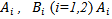
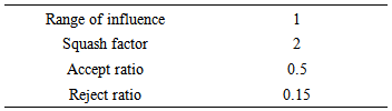
To evaluate the performance of the proposed method in modeling of the Phantom robot, five different variants of Artificial Neural Networks (ANNs) are employed. Phantom robot in New Technology Institute of Iran, see Figure 4, is used. In order to model Phantom robot, a computer program is performed under MATLAB (R2008b) environment. A hybrid–learning algorithm is utilized to train the ANFIS model and the number of epochs is 100. To generate initial Fuzzy Inference System (FIS), subtractive clustering algorithm is applied, and the parameters using in subtractive clustering algorithm are listed in Table 1. Different types of ANNs determined by their training algorithms and their topologies. Training an ANN means selecting a model by adjusting the weights and bias of the ANN from the set of possible models that minimizes the error of generalization performance. According to Lippman’s research [31], three–layer ANNs not only can solve most problems, but also form a complex random limit of decision. Based on this fact, a three–layer ANN was selected using a sigmoid transfer function in the input and hidden layers and a linear transfer function in the output layer, respectively. In this study, three training algorithms were used to train the three–layer ANN model including the well–known Levenberg–Marquardt Back Propagation (LM BP), the Gradient Descent with Momentum Back Propagation (GDM BP), and Gradient Descent with Adaptive learning rule Back Propagation (GDA BP).

Table 1. Parameters of subtractive clustering

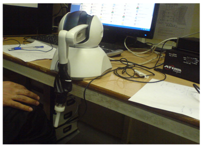Figure 4. Phantom robot in New Technology Institute

The fourth comparison method is Radial Basis Function (RBF), which emerged as a famous variant of ANNs. RBF networks typically have three layers: an input layer, a hidden layer with a non–linear RBF transfer function, e.g., Gaussian functions, and a linear output layer. However, how to select the optimal number of neurons in ANNs and RBF is still an open problem. The last method is Least Square Support Vector Machine (LS–SVR), which it has attracted a lot of attention in modeling and identification [32]. The LS–SVR model is used the RBF kernel in this research due to its superior performance in comparison with the other kernels [33-35].

The model architecture of ANNs model, the RBF network, and LS–SVR model are determined by meticulous trial–and–error to achieve as possible as minimum error rate.

In ANNs models, Tansig transfer function is used in input and hidden layers and Purelin transfer function is used in output layer in both SISO and MISO identification. Moreover, the numbers of neuron in input and hidden layers in SISO and as well as MISO identification are 6 and 8, respectively. Likewise, the minimum error rate is achieved by 150 neurons in RBF network for both SISO and MISO identification. For both SISO and MISO identification, the penalty factor and kernel parameter in LS–SVR method are selected to be 470 and 7.5, respectively.

4.2. Sampling the Model of the Robot

In this study, sampling interval MΔt=0.625 s and time interval Δt=0.00625 s are considered. In order to connect the joint to the computer, we used ieee1394. The applied input and measured output are torque and angle, respectively.

The robot is in open loop form without any controller. Therefore, persistent exciting input is adopted in such a way that stimulated all the various modes of the system. The input signal is a Pseudo–Random Binary Sequence (PRBS). As the collected data may contain false or destroyed information, they are examined in pre–filtering stage after sampling. To investigate the level of output sensor noise, a PRBS with K= 3 periods with the length of M=63 for the first joint, M=127 for both second and third joint are measured. Then, a record of N=KM=189 for the first joint,N=KM=381 data points for both second, and third joints are collected. Figure 5 shows the practical data gathering algorithm.

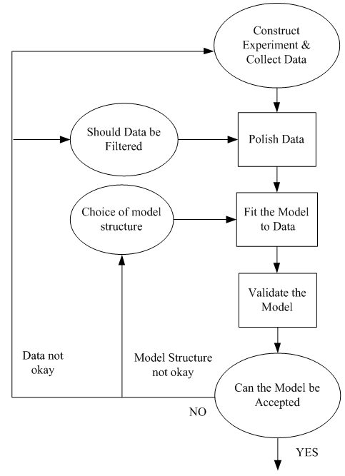Figure 5. Phantom robot practical data gathering algorithm

4.3. Validation Criteria for Model Identification

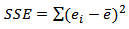
The efficiency of the model is evaluated by comparing the actual values with the approach–estimated ones. Three error measurement indices, i.e., Sum of the Squared Errors (SSE), Mean Absolute Error (MAE), and Mean Square Error (MSE) were used to verify the validation of the ANFIS approach in comparison with other methods in the model identification of the Phantom robot. SSE is used to measure what the difference between each error and its group mean.

(11)

where is the value of the i–th error and is the mean of all the errors.

MAE is a quantity used to measure how close the output is to the actual output. MAE is formulated as follows:

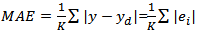(12)

where is estimates the output by the identification methods, is the actual output and is the total number of data.

The Mean Square Error (MSE) is a well–known error measurement, which is frequently used for evaluating the performance of identification methods in the literatures. It is formulated as follows:

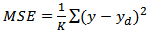(13)

where, is estimatesthe output of the model, is the actual output and is the total number of data. In brief, these techniques will yield an optimal prediction if the values of SSE, MAE, and MSE are close to zero.

4.4. Simulation Results and Discussions

In this section, the results of the comparative experiments between the proposed method and the methods presented in Section 4.1 are discussed. Table 2 shows the results of the comparative experiment in SISO modelling of the Phantom model. This table compares the ANFIS method with other methods based on the criteria listed in Section 4.3. It is interesting to see that ANFIS has higher accuracy than the other methods. For instance, based on MSE criterion, the minimum error obtained for first joint by ANFIS is0.040 and for second joint by ANFIS is 4.8e–5, and third joint by ANFIS is 0.001. The LS–SVR and ANFIS are obtained the same error rate in both first and third joint. ANFIS has lower error rate in second joint. In SISO modeling, LM BP and RBF have the same error rate. Figure 6 shows the input–output relation between robot’s joint in SISO modeling. Furthermore, to demonstrate the advantage of the proposed method in the modeling of the phantom robot behaviour, the results of SISO modelling are displayed in Figure 7.

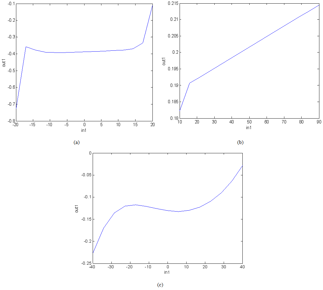Figure 6. The input–output relation in SISO ANFIS predicted model of the Phantom robot, (a) the first input and output of joint, (b) the second input and output of joint, (c) the third input and output of joint

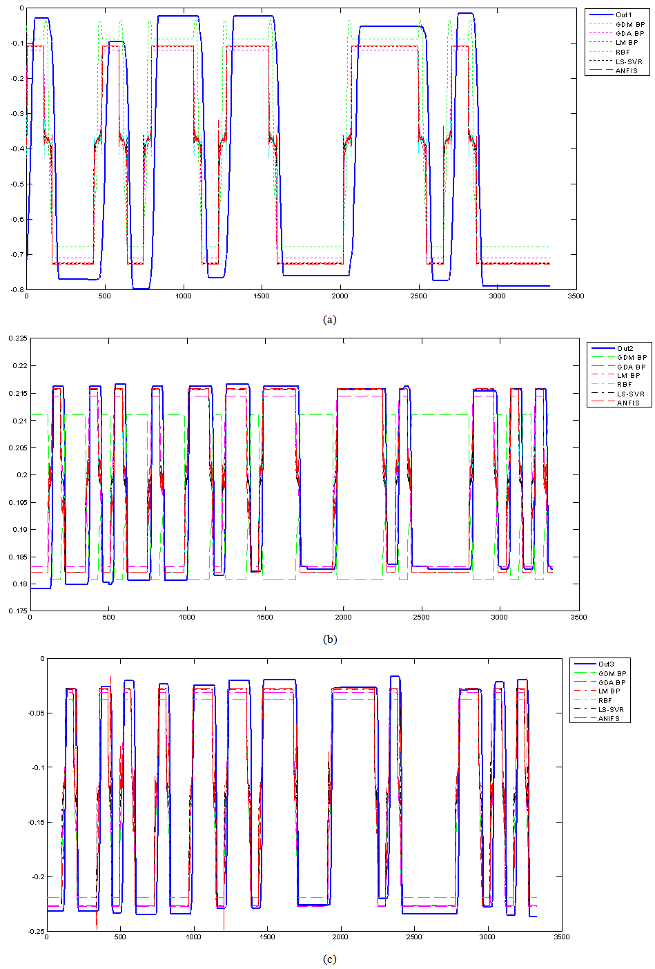Figure 7. Comparison of the SISO ANFIS predicted model and numerical values of the Phantom robot, (a) The first joint output, (b) The second joint output, (c) The third joint output

Table 3 presents the results of the comparative experiment in MISO modelling of the Phantom model. As instance, based on MSE the ANFIS method obtains 0.032 error rate in first joint and 4.0e–6, and 4.6e–5 in second and third joints, respectively. Likewise, LS–SVR is has the same error rate based on MSE criterion for the first manipulator. However, based on SSE and MAE criteria, ANFIS has the lower error rate. In Figures 8, 9, and 10, the input–output relation of first, second, and third robot’s joints are shown, respectively. The modelling results of MISO approaches are shown in Figure 11. In the figure, the modelling of each robot’s arm is shown separately. As shown in the figure, ANFIS approach is superior to other intelligent methods in terms of performance. The model predicted by this method is much closer to the actual model, which is confirmed by the error rate depicted in Table 2 and Table 3 for SISO and MISO models, respectively. By considering the results of the simulations, it can be concluded that the proposed ANFIS approach along with the model selection method is capable enough to be used in other non–linear systems in which various functional states display different dynamic behaviour.

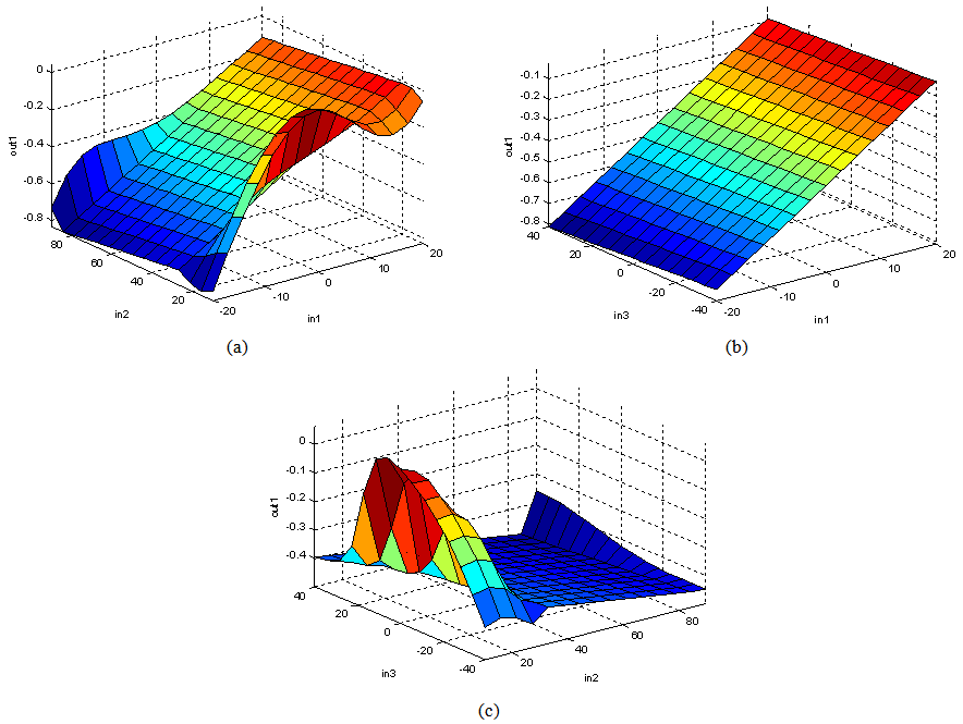Figure 8. The input–output relation in MISO ANFIS predicted model for the first output of the Phantom robot, (a) First output and first and third input, (b) First output and first and third input, (c) First output and second and third input

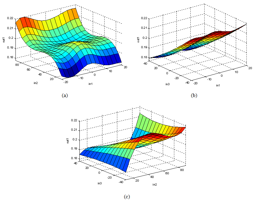Figure 9. The input–output relation in MISO ANFIS predicted model for the second output of the Phantom robot, (a) Second output and first and third input, (b) Second output and first and third input, (c) Second output and second and third input

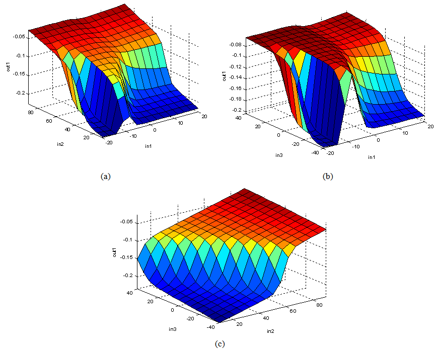Figure 10. The input–output relation in MISO ANFIS predicted model for the third output of the Phantom robot, (a) Third output and first and third input, (b) Third output and first and third input, (c) Third output and second and third input

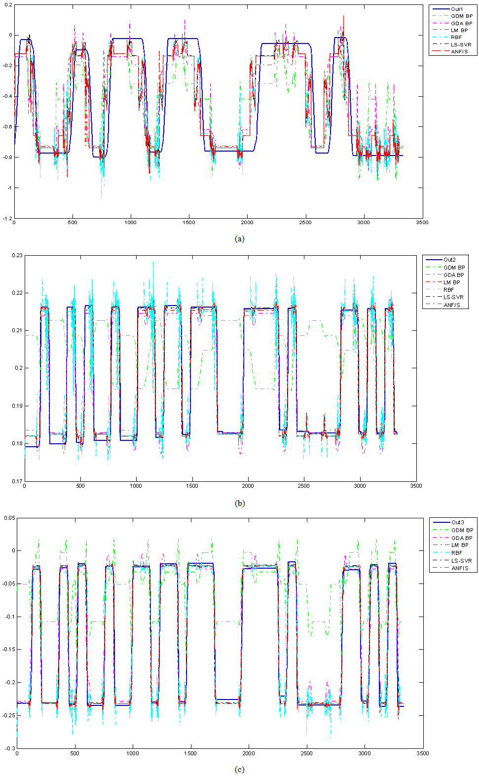Figure 11. Comparison of the MISO ANFIS predicted model and numerical values of the Phantom robot, (a) The first joint output, (b) The second joint output, (c) The third joint output

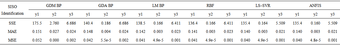Table 2. Comparison performance of SISO ANFIS model for the Phantom robot

Table 3. Comparison performance of MISO ANFIS model results for the Phantom robot

5. Conclusions

Designing and developing a control procedure for industrial robots is highly important, especially considering the accuracy of the robot model, which describes the actual behaviour of the robot. The mathematical model of a robot may be too complicated to be perfectly understood in system identification approaches. In this paper, an ANFIS approach is used for SISO and MISO identification of the model of the Phantom robot. Additionally, a comprehensive comparison of the proposed method was conducted by employing five well–known intelligent identification methods. The simulation results of ANIFS model demonstrated the effectiveness of the proposed approach in terms of statistical measures such as SSE, MAE, and MSE. Given the superior generalization performance of ANFIS method, it can be used in other non–linear systems modeling in which various functional states display different dynamic behaviour.

ACKNOWLEDGMENTS

The authors would like to express their sincere gratitude to the New Technology Institute (NTI) of Iran for the Phantom robot. We are also grateful to Mr. Hamed Ghafari for his comments and suggestions in improving the quality of this paper.