-
Paper Information
- Paper Submission
-
Journal Information
- About This Journal
- Editorial Board
- Current Issue
- Archive
- Author Guidelines
- Contact Us
International Journal of Control Science and Engineering
p-ISSN: 2168-4952 e-ISSN: 2168-4960
2014; 4(2): 27-35
doi:10.5923/j.control.20140402.01
Adaptive Diagonal-Channel Bilinear Filters for Nonlinear Active Noise Control
 Abstract
 Reference
 Full-Text PDF
 Full-text HTML
Li Tan1, Jean Jiang1, Liangmo Wang2
1College of Engineering and Technology, Purdue University North Central, Westville, Indiana, USA
2School of Mechanical Engineering, Nanjing University of Science and Technology, Nanjing, China
Correspondence to: Li Tan, College of Engineering and Technology, Purdue University North Central, Westville, Indiana, USA.
| Email: |  |
Copyright © 2014 Scientific & Academic Publishing. All Rights Reserved.
This paper proposes a novel adaptive bilinear filter with a diagonal-channel structure for nonlinear active noise control. Using the diagonal-channel structure, the diagonal-channel bilinear filtered-X least mean square (DBFXLMS) and recursive least square (DBFXRLS) algorithms are derived. In order to reduce the computational load for DBFXRLS algorithm, the DBFXRLS algorithm with a sequential channel update (DBFXRLS-SEQ) is proposed. Computational complexity for each algorithm is analyzed. Computer simulations demonstrate the control performance improvement of the proposed algorithms.
Keywords: Active noise control (ANC), Nonlinear adaptive filter, Adaptive bilinear filter, Adaptive Volterra filter, Diagonal-channel structure
Cite this paper: Li Tan, Jean Jiang, Liangmo Wang, Adaptive Diagonal-Channel Bilinear Filters for Nonlinear Active Noise Control, International Journal of Control Science and Engineering, Vol. 4 No. 2, 2014, pp. 27-35. doi: 10.5923/j.control.20140402.01.
Article Outline
1. Introduction
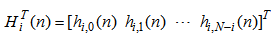
- Active noise control (ANC) has shown effectiveness for controlling disturbance noise, such as noises from engines, blowers, fans, transformers, and compressors [1-5]. The noise types may include low-frequency noise, broadband noise, chaotic noise, and so on. Active noise control system using a linear adaptive controller with a low computational cost is successfully applied. Over the decades, the advances of digital signal processing (DSP) technology have inspired further research in nonlinear active noise control [6-15]. Due to the increase of the speed of DSP processors and the decrease of their costs, many advanced active noise control algorithms may be developed to tackle nonlinear problems in ANC systems and implemented to gain better noise control performance, including the recent development of nonlinear system control with sliding mode techniques [16-17] to solve more general nonlinear problems in the control systems.Active noise control applies the principle of superposition of the primary noise source and the secondary source with its acoustic output being same amplitude and opposite phase of the primary noise source so that a quiet zone can be achieved at the cancelling point. The secondary source is produced by an adaptive filter using a filtered-X adaptive algorithm such as the least mean square (LMS) or the recursive least square (RLS) algorithm. A typical single-channel ANC system using a feed-forward controller scheme is shown in Figure 1.
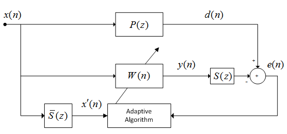 | Figure 1. Block diagram of the single channel ANC system using a filtered-x adaptive algorithm |
 (from the reference microphone or sensor) to generate a cancelling signal
  via a linear adaptive control filter whose transfer function is denoted by
  . The linear adaptive controller drives the secondary speaker to destructively attenuate the primary noise
  . An error microphone is used to detect the error signal
  . The error signal
  and filtered reference signal
  are used by the adaptive algorithm to produce the controller coefficients. Note that
  denotes the primary path between the reference sensor and the error microphone,
  the secondary path between the ANC adaptive filter output and the error microphone, and
  the secondary path estimate which is used to generate the filtered reference signals for the adaptive algorithm.It is well known that linear controllers, especially the linear feed-forward controllers, have been successfully applied to actively cancel the low-frequency noise [1-5]. However, if a noise process to be controlled is a nonlinear and deterministic process such as chaotic noise, or if the primary as well as secondary paths in an ANC system may exhibit the nonlinear behavior, or if the reference signal may have the saturation effect [9-15], the linear ANC system will suffer from performance degradation by using linear controllers. In order to tackle various nonlinear effects, many researchers have developed nonlinear noise control systems using neural networks, normalized Gaussian radial basis function networks, Volterra filtered-X LMS and RLS algorithms, filtered-s LMS, and bilinear filtered-X LMS algorithms [6-15]. The Volterra filtered-X adaptive algorithms [9-10] apply all of the possible products of the delayed input signals to construct nonlinear inputs for the feed-forward controller. The filtered-s algorithm proposed by Das and Panda [11] uses sine and cosine base functions according to the functional-link artificial neural network (FLANN) model to construct the nonlinear inputs. In fact, the nonlinear inputs can be produced using a generalized approach called the function expansion method [12, 13]. To reduce the number of filter coefficients, especially, for adaptive Volterra filters, Kuo and Wu [14] developed a bilinear filtered-X LMS (BFXLMS) algorithm. The developed BFXLMS algorithm is very effective for narrow band noise control when the adaptive bilinear filter is stable during the adaptation and the BFXLMS algorithm converges to the global minimum of the error function. In Kuo and Wu’s original work, the diagonal-channel structure feature described in [18] for the cross terms of delayed input signal and delayed output signal was not considered. When taking into account for the diagonal-channel structure, various improved adaptive bilinear filtered-X algorithms can be developed. The initial results are reported in [15].In this paper, Section 2 will first develop a diagonal-channel structure for bilinear filters. Based on the channel structure, the adaptive diagonal-channel bilinear filtered-X LMS (DBFXLMS) and RLS (DBFXRLS) algorithms will carefully and explicitly be derived. To reduce computations of the developed DBFXRLS algorithm, the sequential channel update strategy according to diagonal-channel signal vectors described in [19-20] are then derived. In addition, comparisons of computational complexities for the developed algorithms are included. Section 3 presents computer simulations to demonstrate the control performance improvement for the situations of using the chaotic noise and primary path having a bilinear model; the chaotic noise and linear primary path; and the saturated reference signal and linear primary path. Finally, conclusions are given in Section 4. The main contributions of this paper include derivations of the diagonal-channel bilinear filtered-X least mean square (DBFXLMS) and recursive least square (DBFXRLS) algorithms, and the DBFXRLS algorithm with sequential update; computational load analysis for each developed algorithm; performance validation using computer simulations.
2. Development of Filtered-X Adaptive Algorithms for Diagonal-Channel Bilinear Filters
2.1. Diagonal-Channel Structure for Bilinear Filters
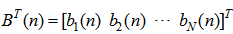
- The relationship between input
 and output
  for a bilinear filter with a memory length of described in [18] is defined below:
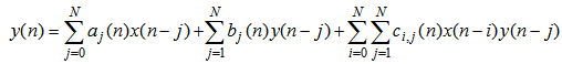 | (1) |
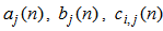 are filter coefficients. Note that
  and
and  have
have  and
and  coefficients, while
  denotes a set of bilinear coefficients and has
  elements. In order to derive a diagonal-channel form, (1) can be equivalently written as:
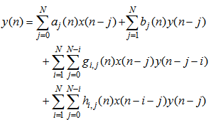 | (2) |
 denotes the bilinear filter channel number and
  designates the time index. Expanding (2) leads to the following summation of all the channel outputs:
 | (3) |
 has
has  coefficients for the channel input signal
  ,
,  has
has  coefficients for the channel input signal
  and so on. Similarly,
  has
has  coefficients for the channel input signal
  ,
,  has
has  coefficients for its channel input signal
  and so on. There are
  channels for the cross terms. Figure 2 depicts the diagonal-channels and signal elements for the case of
  . It can be seen that the signal element in each channel is a delayed term of the previous one.
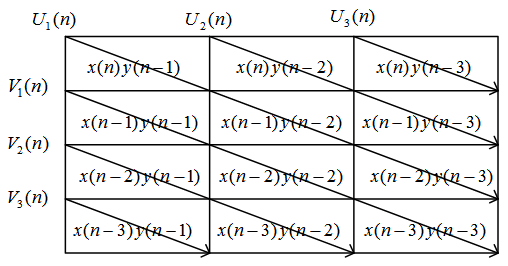 | Figure 2. Cross terms of signal elements and diagonal-channel structure for N = 3 |
 | (4) |
 | (5) |
 | (6) |
 | (7) |
 | (8) |

 | (9a) |
 | (9b) |
 | (10) |
 | (11) |
 channels in total. Both
  and
and  have dimensions of
  . The combined weight vector and reference signal vector are given below:
 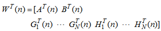 | (12) |
 | (13) |
 | (14) |
 has a dimension determined below:
 | (15) |
2.2. Diagonal-Channel FXLMS Algorithm for Bilinear Filters
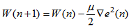
- Using the same approach for deriving the adaptive Volterra filter [8], the adaptive algorithm can be achieved by minimizing the instantaneous squared error using the steepest descent algorithm:
 | (16) |
 is a convergence factor and the gradient estimator is expressed as
 | (17) |
 | (18) |
 , the output of the primary path
  , is the primary noise to be attenuated;
  is the impulse response of the secondary path
  and * denotes linear convolution. Substituting (18) in (17), the error gradient in (17) can further be expressed as
 | (19) |

 | (20) |
 | (21) |
 | (22) |
 | (23) |
 | (24) |
 | (25) |
 | (26) |
 | (27) |
 | (28) |
 | (29) |
 with its estimate
  concludes the DBFXLMS algorithm:
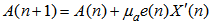 | (30) |
 | (31) |
 | (32) |
 | (33) |
 ,
,  , and
, and  are the convergence factors which control the convergence speed and the stability of the algorithm for updating the feed forward coefficients
  , feedback coefficients
  , and cross term coefficients
  and
and  . Define the signal vector
  as
as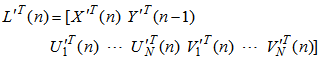 | (34a) |
 ,
,  , and
, and  must satisfy the following condition:
 | (34b) |
 is the maximum eigenvalue of the auto correlation matrix of the filtered input signals,
  . It is also very important to note that the filtered reference signals can be obtained from the following
  channel filters:
 | (35) |
 | (36) |
 | (37) |
 | (38) |
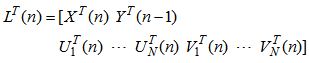
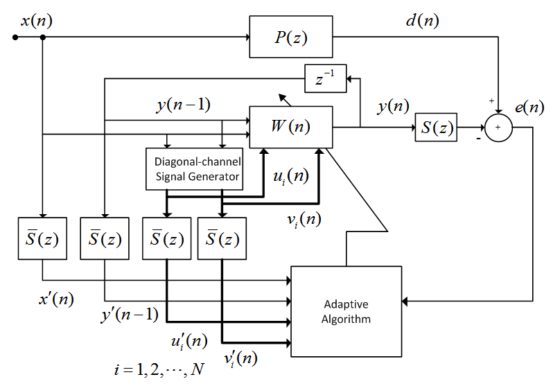 | Figure 3. Diagonal-channel bilinear filtered-X LMS (DBFXLMS) algorithm |
2.3. FXRLS Algorithm for Bilinear Filters
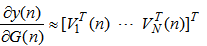
- Using (12) and (13), the standard linear FXRLS algorithm [2] can be modified to the DBFXRLS algorithm:
 | (39) |
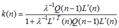 | (40) |
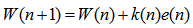 | (41) |
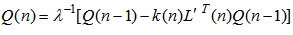 | (42) |

 is the forgetting factor and the initial
  is set to be
  , where
  is the identity matrix while
  is a very small number. As shown in (34), the dimension of
  is in an order of
 . Therefore, the computation requirement for DBFXRLS algorithm is an order of
  . To reduce the computations, the sequential channel update used for VFXRLS and FSRLS in [19, 20] can directly be applied. The resultant DBFXRLS with sequential channel update (DBFXRLS-SEQ) can be expressed as
  | (43) |
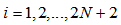
 | (44) |
 | (45) |
 | (46) |
 | (47) |
 | (48) |
 | (49) |
 | (50) |
 ,
,  , and
, and  are the gain vector, inverse of the correlation matrix, and filtered input vector from channel
  , respectively. Again, since the sizes of the gain vector
  and correlation matrix
  for channel
  in the DBFXRLS-SEQ algorithm are much smaller than the one in the DBFXRLS algorithm, the computational load is greatly reduced. On the other hand, the DBFXRLS-SEQ algorithm also prevents the use of a larger size correlation matrix, which may unfavorably cause the algorithm to diverge. Notice that the mean square error function of a bilinear filter is a nonlinear function of its coefficients. It may exhibit local minima such that the algorithm may not converge to the global minimum. The recursive model may be unstable unless the algorithm is carefully designed and filter stability is monitored.
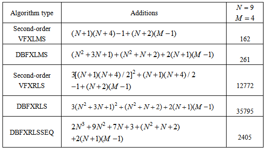
2.4. Computational Complexity
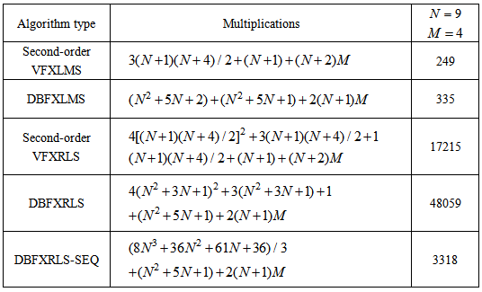
- As shown in Figure 3, the diagonal-channel generator produces
 channel signals, hence, requiring
  multiplications. The output for computing (4) requires
 | (51) |
 | (52) |
 filtered channel signals requires
  multiplications and
  additions, where
  is the number of coefficients in the secondary path estimate
  . These multiplications and additions are the same for all the bilinear filter algorithms.For the DBFXLMS algorithm, the multiplication load for (30)-(33) needs
 | (53) |
 | (54) |
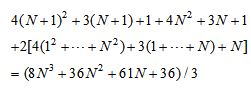
 filter coefficients, it is known that updating (40) needs
  multiplications and
  additions; (41) requires
  multiplications and additions, respectively; and (42) requires
  multiplications and
  additions. The total numbers of multiplications and additions for the RLS algorithm with an input vector size of
  are found as
  and
and  . For the bilinear filter with an input vector size of
  as shown in (15), the total number of multiplications is determined by
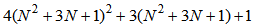 | (55) |
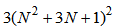 | (56) |
 .
. | (57) |
 | (58) |
 and hence is significantly reduced in comparison to the DBFXLS algorithm with its computational complexity in an order of
 . Among the proposed algorithms, the DBFXLMS algorithm has lowest computational load with an order of
  .
.
|
|
3. Computer Simulations
3.1. Linear Primary Path with Logistic Noise
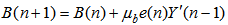
- To demonstrate the performance of the propose algorithms, a linear primary path is assumed to be
 | (59) |
 and its estimate
  with non-minimum phase [10] are the same and given below:
 | (60) |
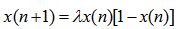 | (61) |
 and
and  are selected. This nonlinear noise process is then normalized to have a unit signal power of
  . The control performance is plotted using the normalized mean square error (NMSE) versus the number of iterations, which is defined below:
 | (62) |
 is the power of the primary noise at the canceling point. In addition, the signal power to noise power ratio (SNR) of 40 dB is used for all the simulations. A memory size of
  is selected for both the second-order Volterra filter and bilinear filter. For the FXLMS based algorithms,
  (linear signal vector) and
  (quadratic signal vectors) are selected for the second-order Volterra filter; for the diagonal-channel bilinear filter,
  ,
,  ,
,  are chosen. Notice that all the step sizes are selected to be less than the corresponding upper bound of
  to ensure the algorithm convergence, where
  is the trace of the cross correlation matrix of the filtered input vector. For the FXRLS based algorithms,
  is selected for the second-order Volterra filter.
  and
and  are selected, respectively, for the DBFXRLS and DBFXRLS-SEQ algorithms. Initial filter coefficients for all the algorithms are set to zero. Figure 4a displays the NMSE’s versus the number of iterations obtained by the VFXLMS and DBFXLMS algorithms. After 500,000 iterations, the second-order VFXLMS algorithm achieves a NMSE value of -30 dB and the DBFXLMS algorithm obtains a NMSE value of -39 dB. The DBFXLMS achieves significantly better performance. Figure 4b shows the NMSE’s versus the number of iterations achieved by the FXRLS based algorithms. As shown in Figure 4b, after 50,000 iterations, the second-order VFXRLS algorithm achieves an approximate NMSE value of -30 dB, while both DBFXRLS and DBFXRLS-SEQ algorithms obtain approximate NMSE value of -40 dB, respectively. It can be seen that the DBFXRLS algorithm has the best performance with a significantly large amount of computations (order of
  ) for each iteration; the DBFXRLS-SEQ offers a compromised solution with the reduced complexity (order of
  for each iteration), and its control performance is better than the one from the DBFXLMS algorithm shown in Figure 4a. Note that the DBFXLMS algorithm has much lower computational complexity with an order of
  for each iteration. Furthermore, the DBFXRLS algorithm shows the fastest convergence rate. However, among these three algorithms, the DBFXRLS-SEQ algorithm gains the benefit from its lower computational load.
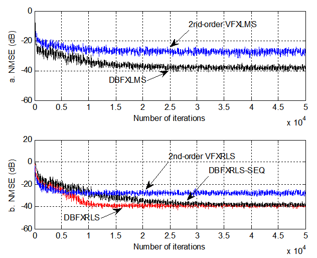 | Figure 4. Performance comparisons: (a) FXLMS based algorithms (2nd-order VFXLMS:  , ,  ; DBFXLMS: ; DBFXLMS:  , ,  , , ; (b) FXRLS based algorithms (2nd-order VFXRLS: ; (b) FXRLS based algorithms (2nd-order VFXRLS:  , ,  ; DBFXRLS ; DBFXRLS  , , ; DBFXRLS-SEQ: ; DBFXRLS-SEQ:  , , ) ) |
3.2. Linear Primary Path with Saturated Narrowband Noise
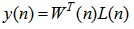
- In the simulations, the measured primary path and secondary path provided in [2] are used. Their frequency and phase responses are displayed in Figure 5.
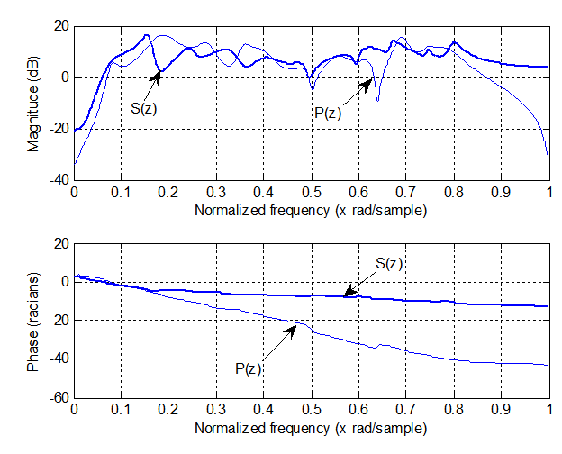 | Figure 5. Frequency responses for the primary path and secondary path used in simulations |
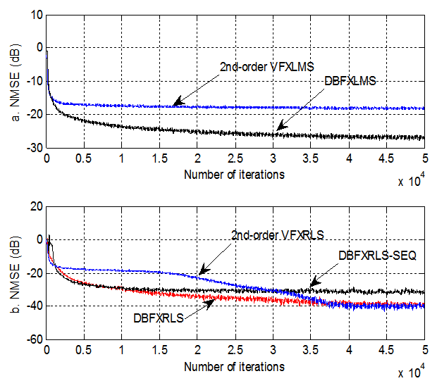 | Figure 6. Performance comparisons: (a) FXLMS based algorithms (2nd-order VFXLMS:  , ,  ; DBFXLMS: ; DBFXLMS:  , ,  , , ); (b) FXRLS based algorithms (2nd-order VFXRLS: ); (b) FXRLS based algorithms (2nd-order VFXRLS:  , , ; DBFXRLS ; DBFXRLS  , , ; DBFXRLS-SEQ: ; DBFXRLS-SEQ:  , , ) ) |
4. Conclusions
- This paper presented a novel adaptive bilinear filter based on a diagonal-channel structure for nonlinear active noise control. Using the proposed diagonal-channel structure, the diagonal-channel bilinear filtered-X least mean square (DBFXLMS) and recursive lest square (DBFXRLS) algorithms are derived. In order to reduce the computational cost for the DBFXRLS algorithm, the DBFXRLS algorithm using a sequential channel update (DBFXRLS-SEQ) is developed. Computer simulations verify the effectiveness of the proposed algorithms.