Paulo David Battaglin, Gilmar Barreto
Department of Semiconductors, Instruments and Photonics, DSIF, School of Electrical and Computing Engineering, FEEC, State University of Campinas, UNICAMP, Campinas, SP, Brazil
Correspondence to: Paulo David Battaglin, Department of Semiconductors, Instruments and Photonics, DSIF, School of Electrical and Computing Engineering, FEEC, State University of Campinas, UNICAMP, Campinas, SP, Brazil.
| Email: |  |
Copyright © 2014 Scientific & Academic Publishing. All Rights Reserved.
Abstract
Instantaneous observability is a method used here to watch a system whose internal states vary very fast. It is a system property which allows us to estimate the system internal states. A discrete computing process which is time-varying can be represented by a mathematical model. This model has linear, discrete, stochastic and time-varying equations which contain matrices and vectors whose elements are deterministic functions of discrete time k. This computing process is performed during a period of time called latency. The process is performed in four steps in sequence, the system states: new process, ready-queue, CPU running, process end. The system propertyinstantaneous observabilitydepends on the pair of matrices {A(k), C(k)} and regards the possibility to estimate the system internal states when the system state equations are known. The problem is the system states are inside and they are not always accessible directly. In this paper we propose a method to determine: the instantaneous observability matrices at discrete time k, the system state estimation and the system latency when the system output measurements are known. We will show when instantaneous observability property comes true, the system instantaneous internal states and latency can be estimated. This is an advantage compared to usual observability method based on static scenarios. The potential application of the results is a prediction of data traffic-jam on a computer process. In a broader perspective, the instantaneous observability method can be applied on identification of pathology, weather forecast, navigation, tracking, stock market and many other areas.
Keywords:
Digital computing process, Instantaneous observability, Discrete time-varying system, Latency, Kalman filtering
Cite this paper: Paulo David Battaglin, Gilmar Barreto, Kalman Filter Applied to a Digital Computing Process to Find Its Latency, International Journal of Control Science and Engineering, Vol. 4 No. 1, 2014, pp. 16-25. doi: 10.5923/j.control.20140401.03.
1. Introduction
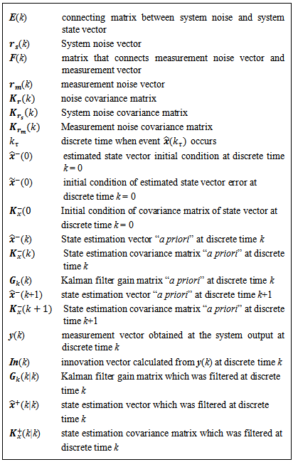
An end-user participates in a teleconference on a personal computer, which is connected through the Internet to another end-user located at a remote place. This teleconference triggers the creation and execution of many computer processes inside this end-user’s personal computer. We will look at a simple computing process which can be represented by a mathematical model that is a system of linear, discrete, stochastic and time-varying equations.Our objectives are: evaluate the end-user satisfaction who is running an application on a personal computer, so that the end-user has a perception that everything is going on like a real time; determinate the latency: when end-user receives fast communications on a personal computer’s monitor screen through sound, image and other messages within the smallest possible time which is the latency; apply the instantaneous observability property on the system of linear, discrete, stochastic and time-varying equations; and apply the Kalman filtering on this system.The current literature issued [1-3] present a ready queue processing time using lottery analysis, an application where the processing time of jobs in ready queue is predicted, and have given their contributions to the field.The approach we will present here is a method to evaluate computing process latency and the latency of each inner state of it through the Kalman filtering in the time domain. The scope of this article is an extent of perception about what is going on inside a computing process as far as time domain is concerned. Each inner state process was estimated using a state space methodology through a Kalman filter which we have built. We have not seen a work like this and for this reason we think it has significance in relation to the other researches. The notation to be used within Kalman filter in this paper is summarized in Table 1. Table 1. Notations
 |
| |
|
2. The Digital Computing Process
Process is a software running program on a digital computer, which can be associated within the operating system internal activities and can be related to end-user programs. A process execution is performed sequentially over time. The process under investigation is performed in a sequence of four steps: new process, ready queue, CPU running, end of process. New Process represents the time of a new process creation  and the connection to the next step. Ready queue represents the time each process remains in a line till it is dispatched to a CPU for execution. This time is represented by a stochastic variable
  associated to dispatching priorities and initial waiting time on a CPU. CPU Running represents the process running time on a central processing unit,
  End of Process represents the time of departure of a process that was executed and its connection to the output and the end-user,
  Each of the four steps can be represented by a mathematical model. The block diagram that represents the process under investigation is shown in Figure 1 below.
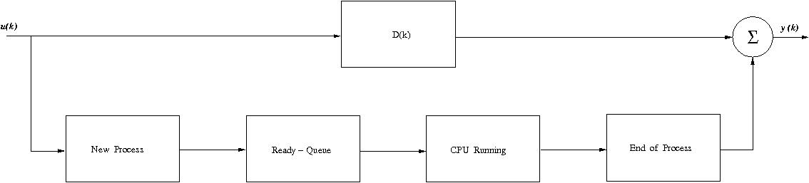 | Figure 1. The block diagram illustration of a digital computing process with four steps in sequence |
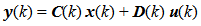
u(k) and y(k) are the input vector and the output vector respectively as well as the matrix D(k) connects the input to the output for control purposes.The output y(k) and input u(k) ratio is a function of discrete time k which can be obtained through a discrete time convolution of the four steps in sequence. The z-transform was applied to this function of discrete time k that relates output and input of process as well as we have got a discrete transfer function that depends on z variable as per equation (1): 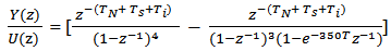 | (1) |
The values of 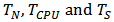 are set up. Then equation (1) can be decomposed by a method of partial fractions,
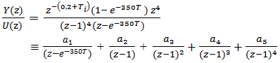
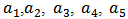 are z-functions to be determined. The partial fractions obtained will allow us to build a block diagram as we can see in Figure 2 below.
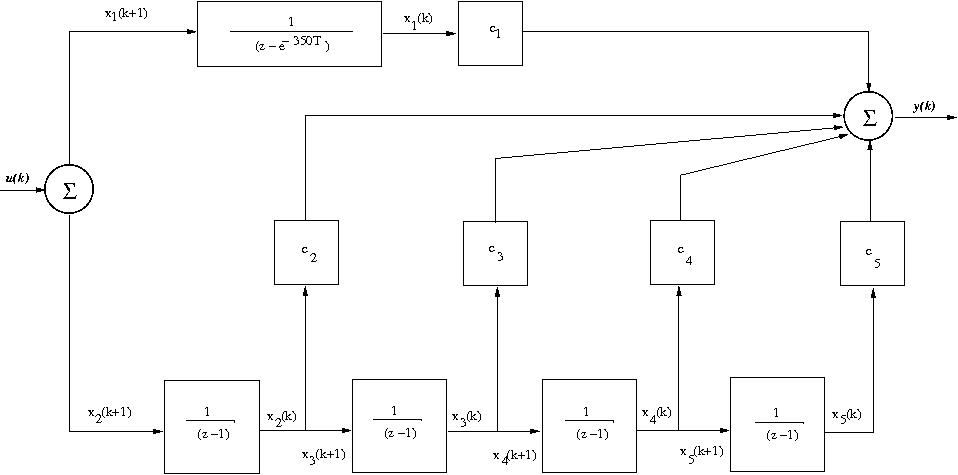 | Figure 2. State variables block diagram of the digital process transfer function |
Based on the block diagram of figure 2 we can write the state equation (2) and measuring equation (3) with state variables in discrete time domain for a digital computing process as follow [4]:  | (2) |
 | (3) |
The vectors  are respectively the system input, the system state and the system output. The matrices
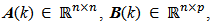
 are respectively the dynamic system matrix, input coupling matrix, measurement sensitivity matrix and input-output coupling matrix which can be seen in reference [9].
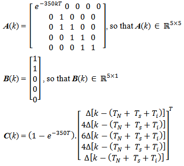 so that
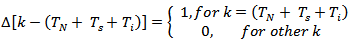
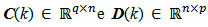
 Kronecker’s delta function for discrete signals.D(k) = 1, so that
  Note that A(k) and C(k) are time-varying matrices and C(k) has a stochastic variable
  The CPU running has two states: waiting for a process and running a process. These estates added to the other three states make A(k)
  . The system input vector u(k) is an impulse train with constant amplitude of 0.07 second over each discrete time interval as well as the solution of Eq. (2) and (3) is the state vector x(k). The system latency is the summation of vector x(k) elements.
3. Instantaneous Observabilty Method
The determination of the instantaneous observability for a linear, discrete and time-varying system depends on time interval over which the instantaneous observability matrix is determined. The system is represented by equations (2) and (3) shown before. The algebraic point of view of instantaneous observability condition it may be presented such as: a linear, discrete, time-varying system is observable, if and only if, its instantaneous observability matrix  has a rank equals to n at each instant of time k, so that n is system state vector dimension [5]. The matrices A(k) and C(k) are time-varying and discrete in time k, for
 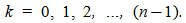 Then the pair of n-dimension matrices {A(k), C(k)} is observable at instant
  if there exists a finite time
  so that,
 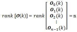 | (4) |
 | (5) |
 | (6) |
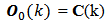
[6] m is the number of row-block matrices so that we have m = 0, 1, 2, … , n-1.The equation (4) is the general shape of the instantaneous observability matrix concerning a linear, discrete and time-varying system. The equation (5) is the generating function of each instantaneous observability matrix block  The equation (6) is the initial block
  of the instantaneous observability matrix. m is the index of block generating function for instantaneous observability matrix, which runs from value zero up to the system order minus one. The instantaneous observability matrix generation is focused on the hypothesis that the linear, discrete and time-varying system is instantaneous observable at the instant k, and there exist times
  so that
  to have valid the equation (4). From equations (5) and (6) we obtain the instantaneous observability matrix blocks to build equation (4) as follow:
 | (6) |
 | (7) |
 | (8) |

 | (9) |
The rank of each stacked matrix in equation (4) is defined as the number of linearly independent column vectors. This is equals to the number of linearly independent row vectors too. Therefore, each matrix block in equation (4) has the dimension then equation (4) rank is
 The global dimension of these stacked matrices is
  n is the number of linearly independent columns and it is also the smallest dimension, and then equation (4) rank is n. Then we conclude the above equation (4) belongs to
  [7]. Consequently, we can build an instantaneous observability matrix set over time shown by equation (10),
  | (10) |
This set we call Set of Instantaneous Observability Matrices of a Linear, Discrete and Time-Varying System. Instantaneous Observability takes into account the possibility to estímate the system instantaneous state vector x(k) based on output measurements, assuming that the state equations (2) and (3) are known.The rank condition for an instantaneous observability matrix of a linear, discrete and time-varying system can be presented in a manner equivalent to the condition of being a positive definite matrix. The product of a transposed instantaneous observability matrix by its instantaneous observability matrix is shown in equation (11) as follows | (11) |
and  The result of this product is a square matrix called Instantaneous Observability Gramian Matrix
  of a linear, discrete and time-varying system. The elements of this matrix are n-dimension vectors result of inner products which vary in time. When the determinant of
  is different of zero, it means this matriz is nonsingular and it is invertible. Hence, there exists a matrix
  so that
  The column vectors of an instantaneous observability Gramian matrix for a given system are linearly independent. Consequently these vectors are mutually orthogonal and they build a base of dimension
  related to Euclidean inner product. This Gramian is a qualitative algebraic characterization of the solution uniqueness. The output vector y(k) has elements which are available and system state equation solution ís possible and unique, and the system state solution is the state vector x(k) [8].Determinant of
  was computed based on equation (10) and Figure 3 has the results over discrete time k.
From Figure 3 below we note the determinant is positive, constant and equals to 45.3079 over discrete time k, concerning the system the equations (2) and (3). It means all column vectors of the instantaneous observability matrix  are linearly independents.
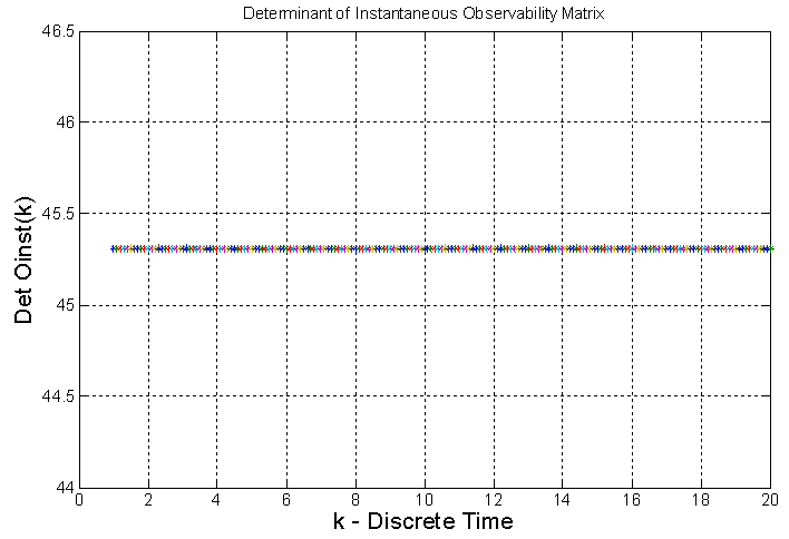 | Figure 3. Determinant of Instantaneous Observability Matrix |
The rank of instantaneous observability matrix was computed and Figure 4 below has the result over discrete time k.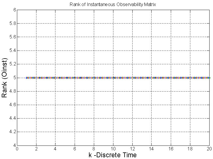 | Figure 4. Rank of Instantaneous Observability Matrix |
From Figure 4 we note the rank of instantaneous observability matrix is equals to five. It shows the system has order five and it is instantaneously full observable.From Figure 5 below we note the instantaneous observability gramian matrix determinant is positive, constant and equals to 2052.83 over discrete time k. It shows all column vectors of the instantaneous observability gramian matrix  are linearly independents and there exists a unique solution for equations (2) and (3) which is the state vector x(k) and its covariance matrix
 Then we have seen the system is instantaneously observable and it means the system internal states can be estimated. The Kalman filter will make this estimation.
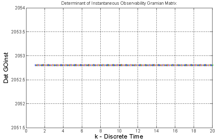 | Figure 5. Determinant of Instantaneous Observability Gramian Matrix |
4. Kalman Filter Applied to a Digital Computing Process
In preparation for applying the Kalman filter to the system equations that represents the digital computing process defined in section 2, we will arrange the Kalman filter equations with the appropriate notation, so as to facilitate a visualization for filtering algorithm. We will use the concept "a priori" which refers to values obtained before the measurement, as well as the concept "a posteriori" that refers to that after obtaining the values measured at the system output. The vectors and matrices with values "a priori" will be represented by a superscript minus "-" as 
 The vectors and matrices with values "a posteriori" will be represented by a superscript plus "+" as
  and
and  Filtering is the processing of y(k) measurement obtained at the system output to improve or refine the estimates of the state
  and
and  at time k. After this, we will obtain the filtered estimates
  and
and  which will propagate. Similarly to the measurement y(k +1), to enhance or refine the estimates of the state
  at time k +1. After this, we obtain the filtered estimates
 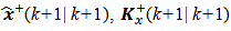 which will propagate. The matrix equations (12), (13) and (14) below represent the mathematical model of the linear, discrete, stochastic and time-varying system; the system Gaussian white noise component
  was added on equation (12), the measurement Gaussian white noise component
  was added on equation (13) and the noise covariance matrix
  is shown by equation (14). These noises are not correlated. Matrix equations (15) to (24) represent the Kalman filter and its initial conditions concerning the values "a priori" and "a posteriori" for each discrete time interval k.• Mathematical model of the linear, discrete, stochastic and time-varying system
 | (12) |
 | (13) |
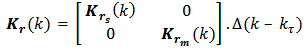 | (14) |
• Kalman filter initialization with initial conditions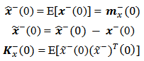 | (15) |
• Kalman filter Gain before measurement | (16) |
• Processing before the measurement-propagation | (17) |
 | (18) |
• Getting the measurement y(k) at the system output and calculate the innovation  | (19) |
• Kalman filter Gain after measurement: filtered Gain | (20) |
• State update to the measurement: filtered state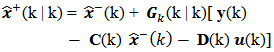 | (21) |
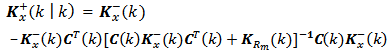 | (22) |
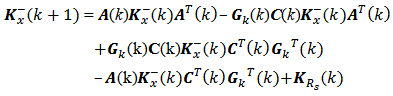
• Propagation of state until the following interval k | (23) |
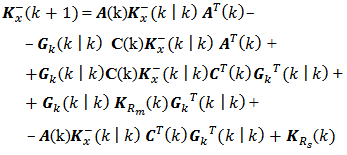 | (24) |
Test: Was the last measure processed?○ If not, go to the equation (19) ○ If so, finish processing the Kalman filter algorithm for digital computing process [9].
5. The Latency of a Digital Computing Process
When an end-user submits an application and sometime later receives fast communications on a personal computer’s monitor screen through sound, image and other messages within the smallest possible time, this time is the latency. The utility of latency is to measure the satisfaction of this end-user who is using an application on a computer, so that the end-user has the perception that everything is happening in real time; when the personal computer receives rapid communication through sound, image and other messages like "a bar of sound intensity" with the lowest latency. In order to determine the latency of our digital computer process, we have set up the initial conditions to run the algorithm called Kalman filter; system noise and measurement noise are generated as Gaussian white noises, the Kalman filter initial conditions as per equation (15) are given, measurements at system output are available, matrices A(k), B(k), C(k), D(k), E(k), F(k) are known. The system input vector will be u(k) which is a train of pulses of two bytes.The four following figures we will see bellow illustrate the “a posteriori” behavior for filter gain, state vector, error of estimation covariance matrix and latency given by the Kalman filter, after the end-user has submitted the application twenty times. The figures have dashed lines which represent discrete values. The numbers to be presented have four decimals. Next we will see the Figure 6 with the five elements of the Filter Gain Matrix "a posteriori" obtained from the matrix equation (20). In these elements the errors on the Gain "a priori" were filtered and the filtering is based on the measurements read at the system output, under the condition of minimum error variance.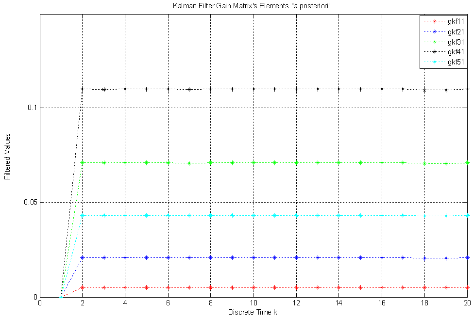 | Figure 6. Kalman Filter Gain Matrix’s five elements which were filtered |
This figure shows the five Kalman Filter Gain Matrix’s elements which have the following values: gkf11(k) = 0,0050; gkf21(k) = 0,0208; gkf31(k) = 0,0712; gkf41(k) = 0,1102; gkf51(k) = 0,0433. These filtered values mean the error covariance matrix has its elements minimized. In other words, the system state estimations have variances which were minimized by the Kalman filtering. The Gain matrix with filtered values can be written as,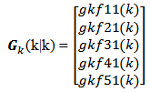 Next we see Figure 7 with the estimated state vector’s five elements "a posteriori" which were obtained from the matrix equation (21). In these elements the estimation errors were filtered based on the measurements obtained at the system output. In this figure the estimated state vector elements have the following values: xestMf11(k) = 0.0247 second; xestMf21(k) = 0.0517 second; xestMf31(k) = 0.1168 second; xestMf41(k) = 0.1361 second; xestMf51(k) = 0.0894 second. The gain matrix is influenced by innovations too and so this matrix and vector of innovations act on the values "a priori" of the state vector, turning them into "a posteriori" or filtered values.The estimated state vector with filtered five elements can be written as,
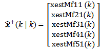 The vertical scales of Fig. 7, 8 and 9 are not the same, in order to facilitate viewing and comparing the amplitudes of mean vector elements, the covariance matrix elements and latency.
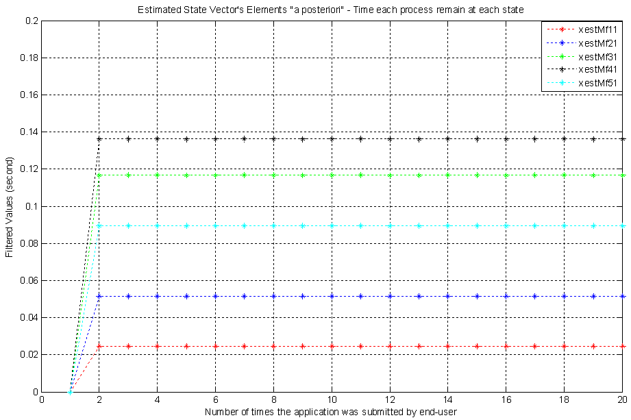 | Figure 7. Five elements of the estimated State Vector which were filtered |
 | Figure 8. Covariance Matrix’s five elements which were filtered |
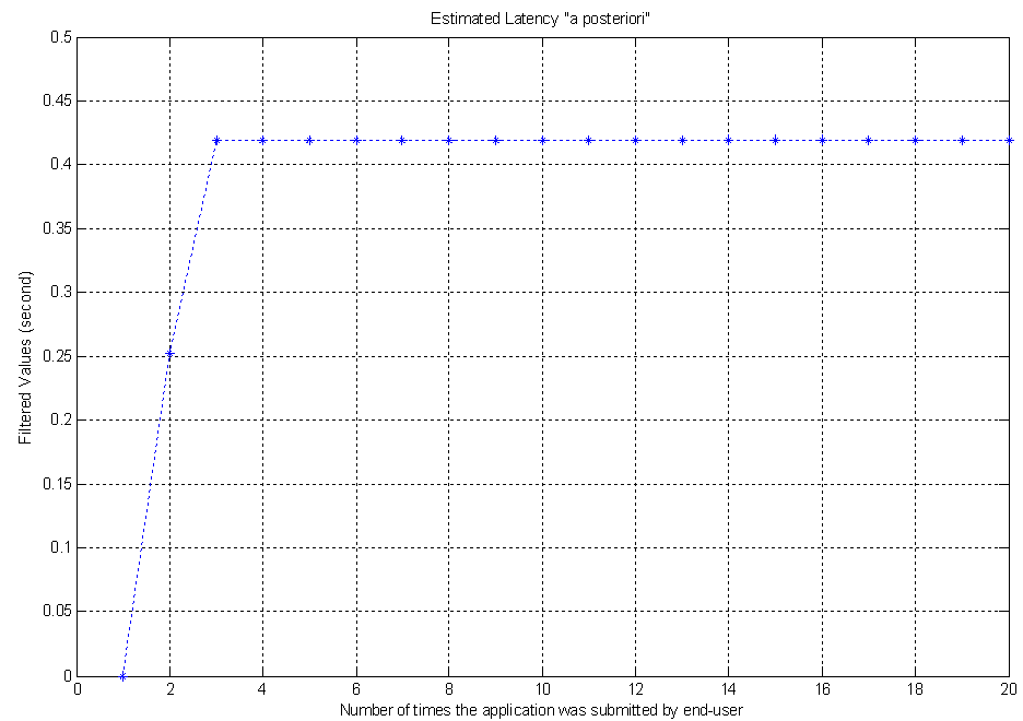 | Figure 9. Latency of a digital computing process under investigation |
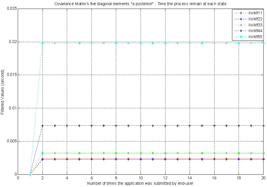
Next we see Fig. 8 with the five elements of the covariance matrix "a posteriori", which were obtained from the matrix equation (22). In these elements the errors of state estimation were filtered based on the measurements obtained at the system output. The elements of the covariance matrix have the following values: KxMf11(k) = 0.0024 second; KxMf22(k) = 0.0023 second; KxMf33(k) = 0.0032 second; KxMf44(k) = 0.0074 second; KxMf55(k) = 0.0198 second. Moreover, as the covariance matrix is time-varying, the time average of the trace of covariance matrix "a priori" equals to 0.0513 second, while the time average of the trace of the covariance matrix "a posteriori" equals to 0.0351 second. In other words, the elements of the covariance matrix converge over the interval.["a priori" → "a posteriori"]. This makes sense because the more measurements are obtained at the system output over the discrete time k, the better the system state estimation.The covariance matrix  with five filtered diagonal elements can be written as
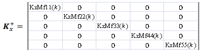 The Figure 9 above depicts the latency which is the sum of estimated and filtered five elements of the state vector x(k). The sum is based on sums of averages theorem [10]. Then this digital computer process latency is 0.4186 second. It means the end-user submits an application and 0.4186 second later receives the result on the personal computer’s monitor screen. If the same application is submitted twenty times, then each of the twenty latencies will be 0.4186 second. The application was submitted twenty times to check the mathematical model and the repeatability of the results.
6. Conclusions
We have seen the system is instantaneously observable at output and it means: the measurements could be obtained at the system output instantaneously and the system internal states could be estimated by Kalman filter instantaneously. The input vector u(k) was given and the measurements at system output could be determined. The Kalman filter equations were built according to state space approach as well as it was applied to the system of linear, discrete, stochastic and time-varying equations which represents the digital computing process. The filter Gain matrix behavior, the estimation of the state vector and the error of estimation covariance matrix along discrete time k were determined through Kalman’s algorithm. We have concluded it is possible to apply the Kalman filter to a digital computing process and estimate its latency on an instantaneous basis.The latency was determined by the sum of the five elements of the estimated and filtered state vector, based on the sums of averages theorem. The end-user expectation about latency will determine the level of satisfaction. If the expectation is not set up by an end-user, then any result can guarantee a satisfaction. If the end-user expectation is less than one second, then the end-user’s satisfaction will be assured here. If the end-user expectation is latency less than 0.4186 second, then the end-user will not be happy. Anyway, the end-user satisfaction level depends on the expectation. The potential application of the results is a prediction of data traffic-jam on computer processes. In a broader perspective, the instantaneous observability method within Kalman filter can be applied on other digital computer processes and other variables than latency can be observed. It is also possible to apply this method to a computer with several CPUs in parallel and an I/O processor, to a several computers like this one connected to a local area network and it connected to a major server, to several major servers connected to a mainframe supercomputer type. Beyond that it can be applied on identification of a pathology, weather forecast, navigation and tracking on ground, water, air and space areas; and stock market prediction.
ACKNOWLEDGEMENTS
We thanks CNPq – National Council of Scientific and Technological Developement – in Brazil for financial support through the doctoral scholarship granted, which made this research possible at DSIF/FEEC/UNICAMP.
References
| [1] | Shukla, Diwakar; Jain, Anjali; Choudhary, Amita. Prediction of ready queue processing time in a multiprocessor environment using Lottery Scheduling, Journal of Applied Computer Science & Mathematics, Number 11, Volume 5, Suceava, Romania, 2011. |
| [2] | Shukla, Diwakar; Jain, Anjali; Choudhary, Amita. Estimation of ready queue processing time under SL scheduling scheme in multiprocessor environment, International Journal of Computer Science and Security, Number 4, Volume 1, pp.74-81, 2010. |
| [3] | Shukla, Diwakar; Jain, Anjali; Choudhary, Amita. Estimation of ready queue processing time under Group Lottery Scheduling (GLS) in multiprocessor environment, International Journal of Computer and Applications, Number 14, Volume 8, pp.39-45. 2010. |
| [4] | Cadzow, James A.; Martens, Hinrich R., Discrete-time and computer control systems, Prentice Hall, New Jersey, USA, 2011. |
| [5] | Kalman, Rudolf Emil; Lectures on Controllability and Observability - Reprint, Centro Internazionale Matematico Estivo - Firenze - Italy, Springer-Verlag, Berlin Heidelberg, Germany, 2010. |
| [6] | Chen, Chi-Tsong; Linear System Theory and Design, 3rd. Edition, Oxford University Press, New York, NY, USA, 2009. |
| [7] | Battaglin, Paulo David; Barreto, Gilmar; Observability of State Space Model in Linear Discrete Time-Varying Systems, Congresso Latino Americano de Control Automatico – IFAC, Lima, Peru, 2012. |
| [8] | Fairman, Frederick Walker; Linear Control Theory –The State Space Approach, John Wiley & Sons, New York, USA, 2000. |
| [9] | Battaglin, Paulo David, Kalman Filtering applied to a Digital Computing Process with a Time-Varying State Space Approach – PhD thesis, DSIF/FEEC, University of Campinas, SP, Brazil, 2014. |
| [10] | Lemons, Don S. (2000). An Introduction to stochastic process in Physics, The John Hopkins University Press, Baltimore, MD, USA, 2002. |
 Abstract
 Reference
 Full-Text PDF
 Full-text HTML