-
Paper Information
- Paper Submission
-
Journal Information
- About This Journal
- Editorial Board
- Current Issue
- Archive
- Author Guidelines
- Contact Us
International Journal of Control Science and Engineering
p-ISSN: 2168-4952 e-ISSN: 2168-4960
2013; 3(3): 81-85
doi:10.5923/j.control.20130303.02
Computational Complexity of Kharitonov’s Robust Stability Test
 Abstract
 Reference
 Full-Text PDF
 Full-text HTML
Kavitha Panneerselvam, Ramakalyan Ayyagari
Department of Instrumentation & Control Engineering, National Institute of Technology, Tiruchirappalli, 620012, India
Correspondence to: Kavitha Panneerselvam, Department of Instrumentation & Control Engineering, National Institute of Technology, Tiruchirappalli, 620012, India.
| Email: |  |
Copyright © 2012 Scientific & Academic Publishing. All Rights Reserved.
Owing to several uncertainties in the modelling of a system, checking for “robust stability” is, in fact, a more practical goal for any designer. In this, instead of a single matrix A, a family of matrices (A + δA) has to be checked for negative definiteness. This led us to the question “How long does a computer take to check the sign definiteness of a family of matrices?” Mathematically, we still have a system of differential equations, but each of the coefficients belongs to certain interval, giving rise to “families of polynomials”. The family of polynomials must be tested to be certain that all the roots lie in the left half of the complex plane. We simply consider the 4 bounding polynomials of Kharitonov and run the algorithms developed above 4 times. Evidently, the savings in computational time is huge. This paper explores the computationally faster algorithm to determine the robust stability of an interval of polynomials.
Keywords: Robust Stability, Kharitonov’s Theorem, Hurwitz Polynomial, Faster Algorithm, Computational Complexity
Cite this paper: Kavitha Panneerselvam, Ramakalyan Ayyagari, Computational Complexity of Kharitonov’s Robust Stability Test, International Journal of Control Science and Engineering, Vol. 3 No. 3, 2013, pp. 81-85. doi: 10.5923/j.control.20130303.02.
Article Outline
1. Introduction
- The robust stability of a linear time-invariant control system containing a plant which has some transfer function coefficients subject to perturbation. The set of transfer functions generated by varying these coefficients in prescribed ranges correspond to a box in parameter space is referred to as an interval plant. The stability of such system is a problem in the theory of robust control with structured perturbations. Kharitonov’s theorem (Kharitonov, 1978) that deals with the stability of an interval polynomial could be appropriately generalized to deal with this problem.The analysis of control systems with parameter uncertainties has generated much interest in the area of robust stability. As uncertainties in system parameters manifest themselves in coefficient variations in the plant characteristic polynomial, many approaches have sought to determine conditions under which one can guarantee that the roots of the perturbed characteristic polynomial lie in a prescribed region, generally the LHP.Several proofs of Kharitonov’s theorem are available in the literarture. An alternative proof of Kharitonov’s theorem on the stability of linear time-invariant continuous systems under parameter variations is presented by Yeung and Wang (1987). The theorem is proved based on the three lemmas. The problem of the robust stability of a linear time - invariant control system containing a plant, some (or all) of whose transfer function coefficients are subject to perturbation within prescribed ranges is described by Chapellat and Bhattacharyya (1989).The proof of Kharitonov’s theorem for the robust stability of interval polynomials using the second method of Lyapunov was presented by Mansour and Anderson (1993). As the Hermite matrix can be used to construct a Lyapunov function to prove Hurwitz stability, then the above result was considered as a Lyapunov - Kharitonov link. Tempo (1992) explored the emerging research area of robust stability and study its interplay with computational complexity. They combine the theorem of Kharitonov with the test of Routh and showed that the number of elementary operations required for the solution of this problem is at most O (n2)In this paper, we present a computationally faster algorithm which runs in O (n), saving the running time by an order when compared to the conventional Routh – Hurwitz (R – H) criterion. This paper explores the computationally faster algorithm to determine the robust stability of interval of polynomials. The robust stability is determined by applying our faster algorithm using row reduction operation.This paper is organized as follows. In section 2 we revisit the Kharitonov’s theorem. In section 3 we shall present our computationally faster algorithm based on the Hurwitz determinant and derive its running time. In section 4 we present several illustrative examples highlighting the saving in computational complexity of the stability problem, particularly when the order of the system is very high. We conclude the paper in section 5.
2. Kharitonov’s Theorem Revisited
- Kharitonov’s theorem is used to determine the stability of an uncertain system by defining four bounding polynomials and applying Routh - Hurwitz test to each of them. It gives a necessary and sufficient condition for all polynomials in a given family to be Hurwitz stable (Callier and Desoer, 1991) In this, the family of polynomials considered is obtained by allowing each of the polynomial coefficients to vary independently within an interval. It shows that stability of this family of polynomials can be determined by looking at the stability of four specially constructed vertex polynomial.
2.1. Theorem Statement
- Consider the set
 of monic real polynomials of degree
  of the form
 | (1) |
 the coefficients are constrained by
 | (2) |
 corresponds to a polynomial of set A, and conversely; thus thinking in coefficient space, we think of
  as parallelopiped in
  whose edges are parallel to the coordinate axis of
  • We say that the polynomial
  is Hurwitz iff
  • We say that the set
  is Hurwitz iff p
 ,
,  , equivalently, iff every polynomial in
  is Hurwitz
 2.2. Hurwitz Polynomials
- The following well known elementary lemma is the basis of our proof.Lemma.1. If the real monic polynomial is Hurwitz, then all its coefficients are positive and
 is a strictly increasing function of
  .2. The real polynomial
  of degree
  is Hurwitz
  Proof:1. Since
  is monic Hurwitz, it can be factored as
 | (3) |
 ’s are the real zeros of p, (hence
  ), and the
  ’s are the complex conjugate pairs of zeros of p, hence
  . The above mentioned equation shows that all the coefficients of p are positive. The fact that arg p
  is strictly increasing is immediate by calculation using this equation, or geometrically obvious by drawing a diagram showing the constellation of zeros in
  .2.
.2.  (a) is immediate since there are no zeros on the
  axis. (b) As
  increases from 0 to
  , arg(j
 increases by
  and that of
  increases by
  . Since there are no zeros in
  , the net increase is
  .
.  Sketch of proof:Suppose that
  had one real zero
  with
with  ; then
  would decrease by
  as
as  increases from 0 to
  . Hence (ii) would be violated since p has degree n, and the net increase in argument of the LHS of (ii) would be strictly less than
  .
.3. Proposed Algorithm
- Given the characteristic polynomial, we first build the Hurwitz matrix
 time. Then, we perform the closed row-reduction operations. The resultant matrix is an upper triangular matrix. An inspection of diagonal elements of resultant matrix for their sign completes the test. This algorithm is applied for all the four specially constructed vertex polynomials.
3.1. Row Reduction Operation
- The well known Hurwitz matrix associated with the polynomial (Guilleman, 1967) is given by
 | (4) |
 determinants are computed, this new criterion needs only one determinant to be computed.It is well known that the sign of a determinant is preserved when certain row-reduction operations, i.e., adding a scalar multiple of another row to a given row, are performed on the square matrix. Further, if these row-reduction operations are carried out on a set of
  rows, resulting in a new set of
  rows, the operations might be said to be closed. Effectively, we might reduce a given square matrix to a triangular matrix via these two operations while maintaining the sign of the determinant. We use the following theorem from (Li, 2007)Theorem:The characteristic polynomial of a square matrix
 ,
,  , where
  , is a Hurwitz polynomial if and only if the Hurwitz matrix above (eqn.4) can be reduced to an upper triangular matrix of the form.
 | (5) |
 are zeros.For the square matrix
  of order
  , the closed row-reduction operations performed at each step may be given by
 | (6) |
 , we obtain the triangular matrix
  . An inspection of the diagonal elements of
  for sign change completes the test.
3.2. Algorithm
- For each of the four Kharitonov polynomial1. Form the Hurwitz matrix
 . 2. Perform modified gaussian elimination r closed row reduction to get
  . 3. Examine the diagonal elements for sign change. 4. If there is a sign change in the diagonal elements, the polynomial is not Hurwitz stable. 5. If all the four set of polynomials are Hurwitz stable, the system is proved for its robust stability. 6. If any one set of polynomial is not Hurwitz the system is not robustly stable
|
4. Illustrative Examples
4.1. Example 1
- Consider the system given in ( Bhattacharyya, Chapellat and Keel, 1995)
 with the coefficients being bounded as
 Verify whether the system is robustly stable.The characteristic polynomial of the closed loop system is
 Since all the coefficients are perturbing independently, we can apply Kharitonov’s theorem. The four Kharitonov polynomials are:1.
  2.
2.  3.
3.  4.
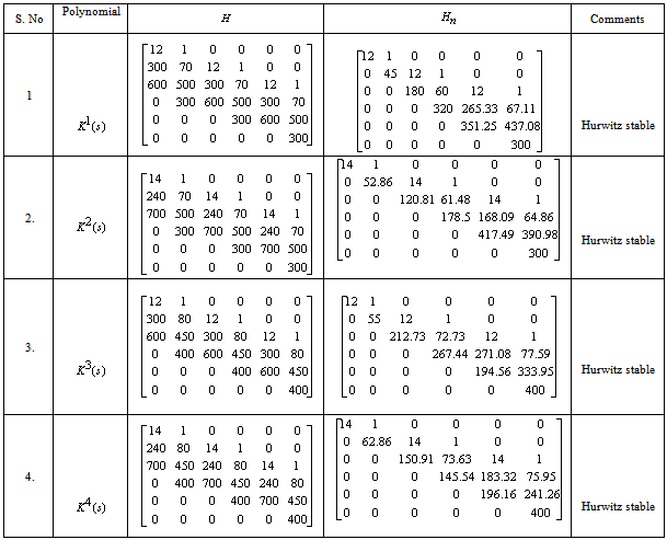
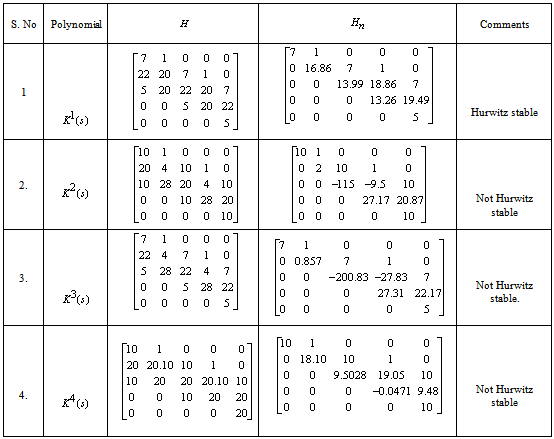
4.  The table 1 shows the Hurwitz stability test of four Kharitonov polynomials. The diagonal elements of
  ,
,  are positive, hence the Kharitonov polynomials
  are Hurwitz stable. The given system is robustly stable.
4.2. Example 2
- Consider a fifth-order interval polynomial given in ( Bhattacharyya, Chapellat and Keel, 1995)
 whose coefficients are specified as follows
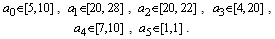 The four Kharitonov polynomials are1.
  2.
2.  3.
3.  4.
4.  From the results shown in table 2, it is clear that, among all the four Kharitonov polynomials, three polynomials are not Hurwitz stable. Hence the given system is not robustly stable.
|
4.3. Computational Complexity
- The computational complexity of robust stability is defined as the minimal number of elementary operations needed to check if the family of polynomials is robustly stable.Given the characteristic polynomial, we first build the Hurwitz matrix
 time. Then, we perform the closed row-reduction operations. While doing this second step, we quickly observe that there are several zeros below the principal diagonal of
  . The number of non-zero elements below the principal diagonal to be made zero, for upper triangularization, follows a simple arithmetic progression. In general, we see that for a given
  , the number of operations needed is
  for some constants
  and
and  . Thus, an otherwise quadratic time complexity has now become linear, thereby saving the computations by an order. The number of operations to test a single polynomial is about
  . In case of robust stability, four polynomials are to be tested for Hurwitz stability. The number of operations is just the four times of the time complexity.
5. Conclusions
- In this paper, we have discussed about Kharitonov’s theorem on robust Hurwitz stability of interval polynomials. We also proposed a computationally faster algorithm to determine the robust stability of the characteristic polynomial. The time complexity of the robust stability problem is greatly reduced by the proposed method. The algorithm may also be demonstrated for its numerical stability, by applying it to the interval of polynomials having irrational coefficients.