1. Introduction

Singular systems are widely seen in electrical and electronic networks, mathematics, chemical processes, economic and neural networks and etc. Accordingly an increasing attention has been dedicated to such systems during recent years[1-9]. However singular systems are called by different names according to their various types of applications. They are known as generalized state space systems in the field of control theory and mathematics, descriptor systems in engineering and economics, differential-algebraic equations in numerical analysis and semi-state systems in the electric circuit fields.

Singular studies are mainly categorized into two main parts. Actually most of the researches on singular systems are performed during 1960 to 1978. These were involved with the equivalency of differential-algebraic equations and the singular systems theory. Since 1980, the behaviour of such systems has also been investigated typically in control theory.

Order reduction techniques and equivalency forms have played an important role in treatment of singular problems in different fields. In fact, usual procedure for dealing with this kind of system is to (either explicitly or implicitly) reduce it to an equivalent regular state space system.

Studies on reduction procedure of singular equations were surveyed by Gantmacher in 1959[4]. Then, in 1966 Polak introduced an algorithm to reduce a differential system to a linear time independent state form[10]. In 1969 Fettweis and in 1975, Desoer and Dervisoglu explained a method for reducing the state equation of algebraic - differential systems in circuit theory[11],[12]. In parallel, Luenberger proposed an algorithm for the state equation reduction of singular discrete systems in 1977. Using Shuffle algorithm, a singular discrete system can be changed to an equivalent system regardless of the infinite impulsive modes in the system response[6]. Besides,[13-19] have made great progress in the field of controllability, observability and stability of singular systems.

All of the above reports use similar definitions based on regular theory of the reduction technique. In essence, an equivalent system representation based on regular theory keeps most of the original system's dynamics except the infinite impulsive modes. Accordingly neglecting infinite modes is the special problem in these ancient reduction approaches.

Indeed Rosenbrock is a pioneer researcher who took the first step in improving the singular equivalency equations by introducing restricted system equivalence (RSE) model based on generalized theory[17]. Although the proposed technique improved the former reduction methods, there were yet some deficiencies involved.

However, Strong equivalency model is known as a desired and flexible model for such systems[19]. Regarding this, the aim of this paper is to modify singular system identification by implementing Strong equivalency in it. As a matter of fact, an inappropriate equivalent model for singular identification may lead to divergence, excessive computation and identification with low accuracy. To avoid these difficulties, primarily a new Strong equivalency model on the singular system is employed and then the identification algorithm is used on the equivalent model. In addition identification process is applied on the RSE equivalent model and results of the two methods are compared.

Outcome of applying the proposed method is found satisfying in comparison with the previous methods. The verification procedure indicates the effectiveness of the proposed equivalence model in simplifying the complexity of singular identification and improving the difficulties involved with the algebraic equations in these systems.

The rest of the paper is organized as follows: in section 2 a general form of a singular system and its problems of identification are described. Section 3 presents singular equivalency approaches and the usual way they are used. Section 4 explains a recursive algorithm of parameter identification. The results of the proposed algorithm and a traditional method are presented through a simulation approach by an illustrative electrical network in section 5. Finally the work is closed by a conclusion in section 6.

2. Problem Formulation

Consider the following representation form of a linear singular system of order n:

(1)

where x(t) is an n dimensional vector of system state variables, u(t) is an m dimensional vector of input and y(t) is the output vector of length k. E, A, B and C are real matrices with appropriate dimensions, considering E as a singular matrix. is the regression parameter vector containing unknown parameters of E, A, B and C.

Signals w(t) and v(t) are the process and the system output white Gaussian noises respectively with zero mean and variances of W and V.

The target here is to estimate accurately the parameters of system matrices in presence and in free of noise.

Considering the singularity of matrix E, impulsive modes usually exist in this type of system. These specific modes cause dependent state space equations. Dependency of the states produce significant troubles meanwhile singular identification process. In fact the initial conditions have to be evaluated by chance in each iteration of the identification algorithm.

The usual alternative to meet the identification criteria here is to reduce the number of non zero initial conditions in order to have less dependent equations. Thus a reliable equivalency transformation based on the generalized theory is needed in the first step of singular identification. Secondly identification process can be implemented on the equivalent model.

3. Singular Equivalency

Singular systems have more complicated form, including not only the finite dynamic modes but also the infinite dynamic and non-dynamic modes. This complication makes singular systems analysis difficult, especially for identification process and the controller design. Singular equivalencies may cope with these difficulties. On the other hand, choosing a sufficient and confident equivalency model relevant to our special work is an important process.

Most of the previous works done on singular systems equivalency are mainly based on the regular theory without paying attention to the structural and dynamical characteristics of equation (1). In fact, those methods are based on transforming the original singular system in (1) to the following state space system of order. The methods are called order reduction methods. See[4],[10] for further information.

(2)

where p=d/dt and D(s) is the polynomial part of G(s) i.e. the transfer function of system (1). Indeed an order reduction generates loss of information which is a main drawback of equivalency based on reduction techniques.

Later Rosenbrock introduced a new equivalency method with the aid of Kronecker form of (sE-A)[4]. Accordingly a bounded equivalency of the system, RSE based on the generalized theory was developed[17].

Canonical Kronecker form of (sE-A) with the existence of non-singular matrices M and N can be described in the Laplace domain as follows:

(3)

(4)

where identity matrices and have r and n-r dimensions respectively, n is the system regular degree of freedom and is the nilpotent matrix with k=n-r index which is equal to singular system index. Vector of state variables can be divided into two following sub vectors:

(5)

where and are regular and singular subsystem state vectors respectively. System (1) can be written in the following Laplace form:

(6)

From the Rosenbrock definition[17], equation (6) of the original system is written in the following RSE form.

(7)

and denote appropriate sub blocks of MB. Similarly and are sub blocks of CN.

This transformation divides the original system into two subsystems. Accordingly important properties of system behaviour at infinity will be preserved. As a result, behaviour of x in the original system will be similar to the state variables behaviour of the RSE system.

Although this approach has superiority over the conventional reduction techniques, there are still some shortcomings. This is due to considering some of unnecessary restrictions on the algebraic subsystem. On the other hand, the two subsystems' parameters should be estimated separately and this produces inaccuracy in identification process.

A kind of Strong equivalency is used including extra constraints over the Rosenbrock equivalency procedure to overcome the mentioned difficulties. Equation (6) can be stated here as equation (8) under the Strong equivalency.

(8)

where M and N are non-singular matrices and . The constraints here are on R and Q matrices. Therefore two systems and are Strong equivalent if and only if standard forms for them are related by Strong operation as in (8).

In addition this should be considered that finding appropriate matrices in this approach is innovative and varies depending on the type of singularity problem.

It can be clearly seen that the Strong equivalency provide one integrated system rather than two separate sub-systems in RSE model. So system can be identified more easily and precisely with the aid of Strong equivalency. On the other hand the Strong model reflects the original systems' information better.

Experiments indicated that this equivalencytransformation is more reliable and effective for identification process than others[19]; therefore this model is employed in this paper in combination with identification algorithm to identify singular system parameters.

4. Identification Algorithm

Recursive Least Square (RLS) algorithm is applied in this case due to its efficiency in parameter identification.

Considering equation (8) and (7), the objective here is to identify equivalent system parameters through the following procedure which is summarized in three steps of:

1. Update unknown vector of parameters by:

(9)

2. Reconstruct the Gain matrix K(t) as:

(10)

3. Finally update the Covariance matrix by:

(11)

where denotes the parameter vector containing estimated values at time t. is the regression vector, and are covariance and gain matrices, respectively. , and number of iterations must be initially defined as initial conditions. , and will be repeatedly updated in each iteration until the estimated parameters converge to the real values via a stopping criteria.

According to the first stage of the algorithm, output y(t) value is needed in each iteration. Output of the system depends on the state variables as well. Therefore initial conditions of the states are required during the process. So inappropriate equivalent model may cause divergence from the real results which may be ensued by excessive time consumption as it happened in identification on RSE model.

In contrary outcomes of identification algorithm on the proposed equivalent model are satisfactory and very close to the real parameters of the original system.

5. Simulation Results

5.1. Equivalency Results

A practical LCR circuit as shown in Fig. 1[20],[21] is transformed to its RSE and Strong equivalent model.

The following equations can be attained using KVL and KCL laws.

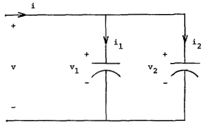Figure 1. A practical LCR circuit in parameter identification

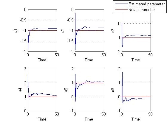Figure 2. Estimated and real parameters-identification on RSE- without noise

(12)

where v(t) is the voltage of the system as output whilst i(t) is the input current source. Equation (12) can be transformed to a state space form in (1), with A, B, C and E matrices as follows:

(13)

with the vector of state variables as follows:

(14)

Matrix E is seen singular, which confirms that the generalized order of the system is 2 (number of passive elements i.e. capacitors). Indeed, system includes an exponential mode at zero frequency and one impulsive mode. Controllability and observability of these two modes are analysed by the following equations from singular controllability and observability analysis[13-19].

Controllability matrix of equation (15) used for finite modes, has a full rank of 4 for the zero frequency mode. Matrix of equation (16) is for infinite controllability analysis with a rank of 6 for this system.

(15)

(16)

Finite and infinite observability of the system is then analysed by equations (17) and (18) respectively.

(17)

(18)

Therefore theses four equations verify that the exponential mode at zero frequency is observable and controllable whilst the impulsive mode is neither observable nor controllable. The latter may cause problem during the identification process due to existence of its initial conditions. After analysing the modes of the system, equivalency methods can be applied on it.

5.1.1. Restricted System Equivalency (RSE) Result

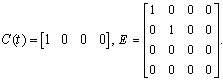
Here, the original system is transformed to its RSE equivalent model to recognize the effectiveness of the proposed model more obviously.

From equation (6), the original system of (13) can be transformed to the following model with state variables of equation (14):

(19)

Regarding equation (7) and (19), the following equations can be attained with unknown state variables of and unknown matrices of .

(20)

To preserve the consistency of the core problem, accept the results here without paying attention to the details. The following results are derived by matching the two state space equations of (19) and (20):

and

(21)

Figure 3. Estimated and real parameters- identification on RSE- without noise

Noticing the results it can be concluded that RSE transformation failed in initial conditions reduction. Its harmful effects on identification process are completely observable in the subsequent sections.

5.1.2. Strong Equivalency Result

As a contribution the following Strong equivalency is employed in this section. Indeed this is inspired form the system analysis. Equation (12) can be manipulated to:

(22)

Accordingly, , and matrices are defined as:

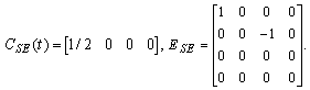(23)

The above representation leads us to a new equivalent system by new state variables of , , and . Input and output of the new system are kept the same as the original system.

By this transformation the initial conditions of the two state variables and exactly become zero. This is an advantage of the proposed equivalency for accurate singular identification in purpose of representing the system just by input-output data. This is because input-output data of the system is mainly used in the identification process.

5.2. Singular Identification Result

In the second step RLS identification is applied on the two equivalent models of previous section.

5.2.1. Identification on RSE Model

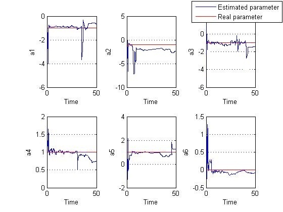
In this case, covariance matrix P(0) is initially chosen as . The two figures are resulted with and without v(t) and w(t) noises respectively. V and W variances are selected as 0.9.

Besides the process is time consuming the final value of the parameters had not arrived at its optimum point. In addition initial conditions are chosen so that divergence does not occur. However it surely happens through an identification of a more complicated singular system.

From Figure 3, noise trace can be completely observed and the final values are not admissible.

5.2.2. Identification on Strong Equivalent Model

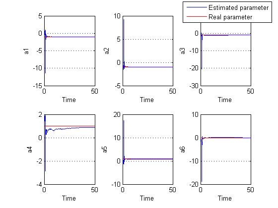
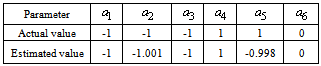
Parameters of the Strong equivalent model in (23) are estimated by RLS algorithm as well. 500 input output samples are used in this algorithm and the initial estimates for the parameters are taken as zero (a possible assumption according to the Strong equivalency). The covariance matrix P(0) is initially chosen as with appropriate dimensions.

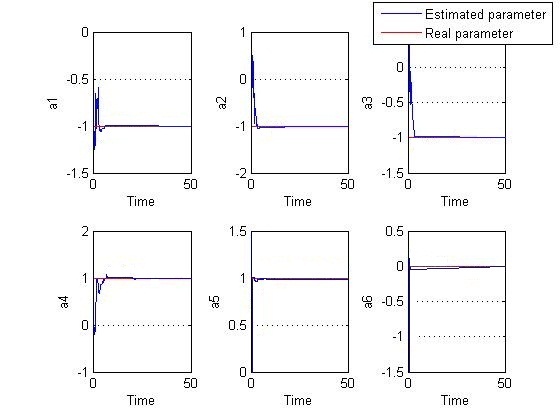Figure 4. Estimated and real parameters-identification on Strong equivalency- without noise

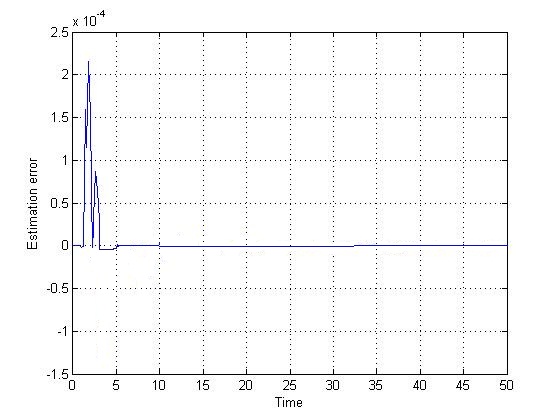Figure 5. Estimation error- identification on Strong equivalency-without noise

Results are achieved in two different cases with and without noise, considering V and W variances as 0.9. Results of using PRBS input free of noise are shown in the following graphs.

From Figure 4, it can be observed that convergence of parameters identification on Strong equivalency is perfect. Estimation error and output tracking results are also found satisfactory from the next two graphs.

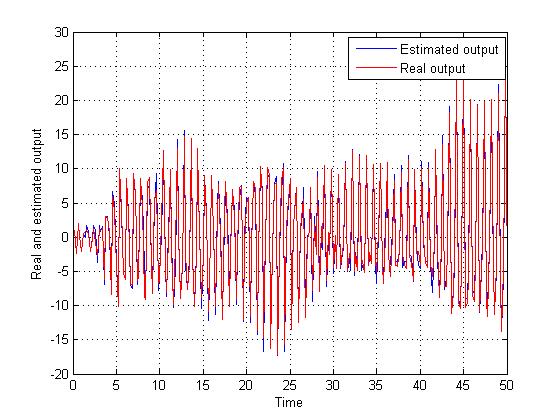Figure 6. Output tracking- identification on Strong equivalency-without noise

Figure 7. Estimated and real parameters-identification on Strong equivalency with noise

Parameters identification results of the proposed method in presence of Gaussian white noise can be seen in the following graphs.

However noisy data produces fluctuations in the outcomes, identified parameters finally converge to the actual values in Figure 7. The estimation error and output tracking results of Figure 8 and 9 show fluctuating patterns, but in a satisfactory accuracy.

Final results of the proposed procedure on the singular system are summarized in the following tables:

Table 1. Estimated Values of Parameters in Free Noise Case- Identification on Strong Equivalency

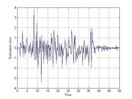Figure 8. Estimation error-identification on Strong equivalency- with noise

Figure 9. Output tracking- identification on Strong equivalency-with noise

Table 2. Estimated Values of Parameters in Presence of Noise- Identification on Strong Equivalency

Theses results confirm the significance of the proposed algorithm in comparison with those obtained in Figure 2 and 3.

Preference of the Strong equivalency is made by including extra constraints to the traditional Rosenbrock's RSE method. This model ignores unnecessary restrictions related to unnecessary initial conditions and improves the troublesome conditions of the system. However this successfully considers infinite mode aspects. In particular, applying the proposed equivalent model within the parameter identification process moderates singular identification difficulties which are caused by algebraic equations.

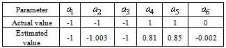
6. Conclusions

An identification technique is implemented in this paper to identify singular systems. Furthermore an appropriate singular equivalency is proposed within the identification algorithm.

The proposed equivalency method is based on restricted system equivalency (RSE) with extra constraints, which provide more accurate equivalent model with fewer initial conditions. Thus, the convergence speed of the identification process is improved in comparison with the previous approach. Significance of the proposed equivalency in combination with the identification algorithm is shown through a simulation study on a 2^nd order circuit. It is seen that estimated values are finally converged to the actual original parameters with fewer estimation error even in presence of white Gaussian noise. The proposed approach also needs less information about the initial values due to transformation of system states to new equivalent states. This new form guarantees the convergence of the identification algorithm by transforming the state variables with zero initial conditions. Simulation results from the new and the traditional methods signify the performance of the proposed equivalency technique in combination with the identification procedure.