1. Introduction

Modern logistics systems pose high demands on mobile transportation, transport vehicles have to be agile, precise and safe. Omnidirectional wheels provide holonomic movement capabilities, allowing vehicles to change their direction of movement, without changing their orientation. This superior maneuverability makes them an attractive choice for logistic vehicles.

The invention of these special wheels dates back to the seventies[1], and they have been used in countless applications both by hobbyists, industrial companies and researchers since then. They have been successfully used in forklifts and other transport machines like the Sidewinder from Airtrax, or the OmniMove platform family from KUKA Robotics and others[2]. They also attract a considerable amount of researchers, who strive to enhance their mechanical capabilities and control algorithms[3],[4],[5]. Figure 1 demonstrates some of the various applications in which they are being used today.

Their advantages however come at a price: they require complex mechanical design, independent drivetrain for each wheel and smart control algorithms.

1.1. Motivation

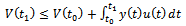
Omnidirectional wheels consist of several – usually rubber coated – rollers around the wheels circumference, the most popular angles are 45° and 0°, the first is usually called Mecanum, or Swedish wheel (Figure 2.), the latter is usually called Omni-wheel. The rollers are spinning freely, only the main axis is powered. Basically they can only exert force parallel to the rotational axis of the roller touching the ground. Because of this they have no self aligning moment, or side force generation capabilities, so they do not keep their rolling direction when pushed or braked, as opposed to a vehicle with conventional tires.

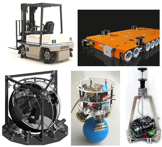Figure 1. Examples for the use of omnidirectional wheels1

Since the load distribution and mass of a transport robot changes each time the cargo is changed, it is quite hard to predict actual load distribution, and in consequence, the resulting friction forces during a braking maneuver. Unbalanced forces generate a torque around the center of gravity, turning the platform, until equilibrium is reached and the platform stops. This is illustrated on Figure 3 showing a simulation of a Mecanum wheeled forklift from above. Three snapshots of the movement can be seen: start of braking, mid braking and final orientation before stopping. The blue arrows, starting from the wheel centers represent tire forces, the yellow arrow at the platform center is the instantaneous velocity vector. Clearly this behavior is undesirable for the operator, as it is unexpected, therefore dangerous. It is easy to see this movement leading to an accident in a narrow aisle.

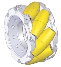Figure 2. Cad drawing of a mecanum wheel[6]

The first part of this article presents a model of a general omnidirectional platform, then the proposed controller is described. The second part of the article shows simulation results demonstrating the disturbance rejection capabilities of the proposed control law.

Figure 3. Brake induced swerving of a Mecanum platform

2. Controller Design

2.1. Problem Description

To be able to find the most suitable control methodology for the problem at hand it is important to find an appropriate description of the system. Friction force generated at the wheels of a braking vehicle always opposes the velocity of the contact patch of the wheel, and its magnitude depends on the intensity of braking, wheel load and the contact properties of the wheel and the ground. This dependency can be described by appropriate wheel and ground models, as accurately as needed, however the result will be only as accurate as our knowledge of instantaneous load distribution and local ground characteristics, which are hard to measure. The load dependent effect is nonlinear, it is often approximated with a negative quadratic function[7].

2.1.1. Kinematics of the General Omnidirectional Vehicle

First let’s consider the kinematic equation of a general omnidirectional platform. This part of my article builds on the work of Indiveri[8], however I made some notational changes. Figure 4 shows the general kinematical model of an omnidirectional platform, three wheels are shown, for the sake of clarity, but the model is true for any number.

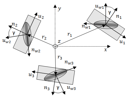Figure 4. Kinematics of the general omnidirectional vehicle

All axes are considered parallel to the ground except for of the local coordinate system and , the unit ground normal pointing the same direction. Let N stand for the number of wheels, then the wheels are indexed by . denotes the position vector of the center of the wheel contact on the ground. The rollers touching the ground are illustrated by the shaded ellipses. The unit vector is parallel with the roller axis, that is the active direction of the roller. is the tangent velocity direction of the roller – that is the passive direction – associated with the rotation around . All wheels are assumed to be identical with the same radius R. The unit vector is the unit vector along the wheels axis of rotation, is the tangent velocity direction of the wheel, as it is rotating around . Lets denote the platform center velocity with and magnitude of angular rotation with The angular velocity points in the direction of .

After a short derivation² the kinematic equations turn out to be the following:

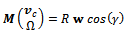(1)

where

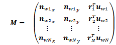(2)

With these equations any desired vehicle velocity can be implemented, given proper wheel angular velocities if:

→ i.e. roller axes are not parallel to wheel axes, which would render the wheel incapable of generating movement

→, this corresponds to controllability of the system

2.1.2. System Dynamics

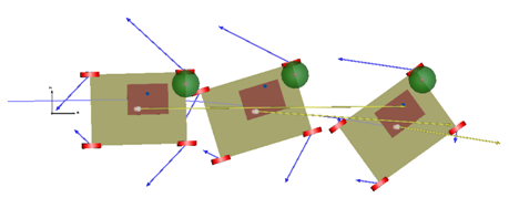
Forces and velocities of an omnidirectional platform during braking are demonstrated through an example of a Mecanum platform braking with nonzero angular velocity – Figure 5. It is assumed that the vehicle moves on a flat surface, consequently it has three degrees of freedom.

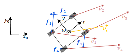Figure 5. Forces and velocities during braking – illustration on a Mecanum platform

The system to be controlled is a MIMO system. Its state equation can be written in the general form:

(3)

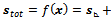
where the usual notations are used – is the state vector, is the input and is a nonlinear function. In the case of an accelerating mechanical system, the state vector consists of resulting linear and angular velocity of a reference point. However for this particular case – a braking omnidirectional platform – it is more practical to also include wheel center velocities: These can be derived in a simple way from platform center linear and angular velocity.

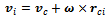(4)

where is the vector pointing from the platform center to a given wheel center.

The input vector consists of a function of the friction force of the wheels and driver input. For the time being let’s assume a constant driver input . System parameters do not change frequently, only when the payload is changed, therefore we can consider the system autonomous, or time invariant. The main dynamical equations can be derived from Newton’s law:

(5)

(6)

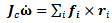
These equations are written for the geometrical center of the vehicle. Even these simplified equations contain various uncertain parameters, such as mass and inertia tensor of the vehicle. Both can change with the load. Further uncertainty is added by the unknown magnitude of friction forces. They are generated to oppose wheel velocity and point in the active direction of the wheel i.e.:

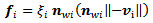(7)

where is a nonlinear function describing dependence of the friction force on wheel load and ground characteristics, for a given driver input i.e. pressure on the brake pedal. is a unit vector pointing in the direction of the roller axis, is a unit vector pointing in the opposing direction of the velocity of the given wheel center. See Figure 4 for notations.

Another important property of the system, that it is strongly cross coupled, all inputs have an effect on all state variables. This follows from equation (2).

2.1.3. Feedback

Measuring the state variables and is not a straightforward task for omnidirectional vehicles, because wheel rotation based methods, frequently used for vehicles with differential, or Ackermann drive would introduce large errors. I assume them to be measurable, for example by a method described in[9], which is especially suited for omnidirectional platforms. This method works much like an optical mouse, however with greater speed range and accuracy than similar works from the literature[10],[11]. can be calculated using equation (4).

2.1.4. Control Goals

In the previous sections I discussed the behavior of the plant and my conclusion is that even according to a simplified model, nonlinearities and parameter uncertainties due to unknown loads and changing ground characteristics make it impossible to prescribe an exact trajectory during braking. Instead of giving an exact trajectory the task can be handled by finding a compromise and describe the goal qualitatively. In the case of a braking omnidirectional vehicle the control goal is twofold:

Goal 1: it is important to avoid directional change in the platforms movement

Goal 2: obviously it is also important to try and stop the platform as soon as possible

The goals are simple but several problems pose difficulties in reaching them:

→ Since the wheels cannot be turned, the direction of force they generate only depends on the velocity direction of the contact patch, therefore the only option to assert control is to modulate the braking force.

→ Force generation is passive in a sense that it can only act to decrease velocity, and not to increase it.

→ Generally the friction forces of the wheels are not parallel with wheel velocities, therefore they will act to divert the platform from its original path, making the two goals contradictory.

→ From equations (1), (2) it is clear that any wheel effects both components of and consequently it is generally not possible to change a single degree of freedom of the platform independently.

The control loop is shown on Figure 6.

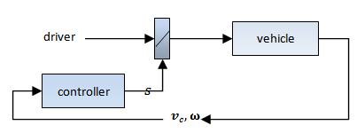Figure 6. The control loop

2.1.5. Applicable Control Discipline

Because of the uncertainties and nonlinearities present in the system I decided to apply a nonlinear control approach. When controlling real dynamical systems uncertainties and disturbances in both the system model and the variables are a common problem. Effects of these uncertainties have to be taken into account in the controller design as they can severely impair control performance or even cause instability. Control of dynamical systems in the presence of heavy uncertainties has become an important subject of research. Due to the efforts made in this field many different approaches made considerable progress, such as nonlinear adaptive control, model predictive control and others.[12],[13],[14] These techniques are guaranteed to reach the control objectives in spite of modeling errors and parameter uncertainties.[15]

Imprecision may come from actual uncertainty about the plant, for example because of unknown parameters, or they might come into the model on purpose by using a simplified representation of the system’s dynamics. These uncertainties are classified as

→ structured - or parametric

→ unstructured - or unmodeled dynamics

The first kind is actually included in the terms of the model, the second corresponds to underestimation, or oversimplification of the system order.

Sliding mode control belongs in the family of robust control, because it is extremely tolerant of parameter inaccuracies. It is characterized by high simplicity. It utilizes discontinuous control laws to drive the system state trajectory onto a specified surface in the state space, the so called sliding or switching surface, and to keep the system state on this manifold after reaching it. Evidently this approach only works when the control input is designed with sufficient authority to overcome the uncertainties and disturbances acting on the system. The main advantages are, that while the system is on the manifold it behaves like a reduced order system and system dynamics are insensitive to uncertainties and disturbances[16].

All these great advantages however come at a price, good performance can only be achieved with extremely high control activity. This results in the so called chattering effect, which is the result of excitation of high frequency components of the system. Ideally control activity has an infinite switching frequency, which in real life applications is a high but finite frequency. High control activity also causes wear and tear of mechanical components. For further reading the reader is referred to:[17],[16],[15],[18] and others.

Formally the problem can be described as follows[15]: Let’s consider the following nonlinear system

(8)

where and . The discontinuous feedback is given by:

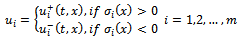(9)

where is the -th sliding surface, and

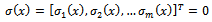(10)

is the dimensional sliding manifold.

The control problem consist of developing the functions and the sliding surface , so that the closed-loop system exhibits sliding mode.

A sliding mode exists if, in the vicinity of the sliding surface the velocity vectors of the state trajectory are always directed towards the surface. In consequence if the state trajectory intersects the sliding surface, the value of the state trajectory remains within a neighborhood of the surface.

2.2. Omnidirectional Brake Assist

The idea behind sliding mode control is to constrain the plant to a prescribed trajectory – the sliding manifold – by choosing the control gains, to drive the state variables towards it. These considerations mean that brake modulation has to depend on the direction of the friction force, if it drives the platform towards the desired trajectory then it needs to be applied, otherwise, the wheel needs to be rolling free. To construct the sliding surface we have to consider the nature of trajectory we would like to track. Since the magnitudes of the forces are uncertain the trajectory cannot be defined as an exact function of time. At the moment when braking starts the platform has initial velocities, the platform has to gradually lose its angular velocity and it cannot gain velocity in the direction perpendicular to i.e. it cannot divert form the trajectory before braking.

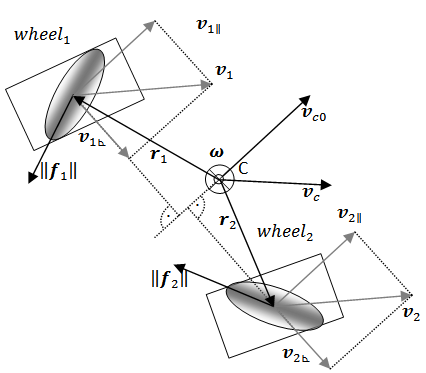Figure 7. Projections of wheel velocities on the initial velocity vector during braking

To translate these considerations into control rules the sliding surface can be written in the following form for each wheel:

(11)

where the three components correspond to wheel velocity components parallel and perpendicular to and a component due to . My approach is based on the property that each component signifies whether the given –-th – wheel is able to decrease that velocity component, therefore the control law can be constructed to apply the -th brake when its corresponding function is negative:

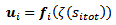(12)

where

(13)

Components of can be calculated the following way:

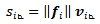(14)

where is the projection of on the direction of the roller axis of the wheel. Similarly

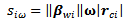(15)

where is the distance from the platform center to the wheel center, and

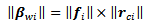(16)

is the direction of the torque, or angular acceleration generated by and the direction of are known from the geometry of the platform and they are generated to oppose the corresponding instantaneous wheel center velocities.

is a different matter, the previously discussed two components change from wheel to wheel, the parallel component however can be decreased by any wheel in most cases, so if we calculate it from vector projections as in the case of we interfere with Goal1. Let us insert a weighing function in the equation as follows:

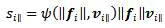(17)

where is the projection of on the direction perpendicular to the roller axis of the wheel, is a weighing function. The best way to define it is to make it angle dependent, large when the given roller is parallel with the velocity vector of its center – most efficient braking direction – and small otherwise. A suitable function I used is:

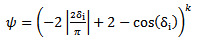(18)

where is the angle between the roller axis of the -th wheel and the parallel component of the wheel center velocity, is an odd integer, that scales the steepness of the function.

Note that all coefficients in the control equation are defined by platform geometry, that is considered to be constant and known in advance. vectors are measured by feedback sensors.

2.2.1. Controller Characteristics

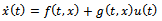
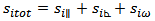
For every control system it is important to show that the closed loop system is stable and that it converges to the prescribed trajectory.

Let’s summarize the control strategy developed in section 2.2. A state dependent error function is defined for the platform, with three components corresponding to three degrees of freedom. The individual brakes on the wheels are switched on and off according to the sign of this error function, as described by equations (12) and (13).

To find out if the closed loop control system is stable I decided to use the so called passivity approach[16] (p. 436). The passivity approach means that if the components in the feedback connection are passive in the sense that they do not generate energy on their own, then it is intuitively clear that the system will be passive. Generally a system is called passive it there exists a storage function , such that for all

(19)

where is the system output and is the input respectively. This equation simply states, that the energy of the system consists of the initial energy plus the supply rate If the equality holds, the system is lossless, if it is a strict inequality then the system is dissipative. For example energy is lost because of friction in mechanical systems, because of heat exchange in thermodynamical, or because of heat generation in electrical systems.

If we set the feedback to where is a positive gain then it is guaranteed that the system energy remains bounded, thus the feedback system is stable. Considering an omnidirectional platform in the context of my brake assist system, energy is stored in the form of kinetic energy. This can be written in the following form:

(20)

considering the linear and rotational kinetic energies. The “supply rate” – in this case would be more appropriately called the “dissipation rate” – is the product of friction force and velocity which is essentially the power dissipated by braking the wheels. The goal of the braking maneuver is to drive the kinetic energy to zero. Brake forces are always generated to oppose movement causing negative acceleration. Since no energy is put in the system by the brake forces, it is evident that the system is passive and the inequality (19) holds true for time instants. However for a braking maneuver a strict inequality is needed for the vehicle to stop in a reasonable distance, which means that if we neglect small frictional effects such as rolling resistance and bearing friction etc. a strict inequality can only be achieved if it is guaranteed that:

→ at least one brake is actuated at any time instant

→ with its active direction at an angle other than to the direction of movement

The second criterion is guaranteed by design, if the vehicle is created so that the rank of in equation (2) is 3, so that the vehicle is in fact useful. The first criterion means that the error function of at least one wheel has to be negative at all times. This is easily guaranteed if we add a rule for the controller that turns every brake on if

3. Simulated Results

To demonstrate the capabilities of the brake assistant, I created a configurable omnidirectional wheel model[19]. The model is based on the well known Rill tire model[7], however its force generating capabilities have been changed to reflect the characteristics of a given omni-wheel. Figure 8 shows a simple sketch of the idea behind the transformation, slip is calculated in the “active” direction i.e. the direction of the axle of the roller on the ground, then driving forces are calculated according to this modified slip. Forces in the free-rolling – “passive” – direction are neglected for sake of simplicity. The advantage of the underlying Rill model is that wheel parameters have physical meaning, they correspond to material stiffness, damping etc. thus they can be set reasonably well by educated guess, as opposed to other tire models where the parameters have to be set by measurements.

Figure 8. A regular tire model with modified slip and force characteristics

I created two simple platforms using Modelica³ language in the Dymola simulation environment. These are the most preferred omnidirectional configurations, their rendered images are shown on Figure 9.

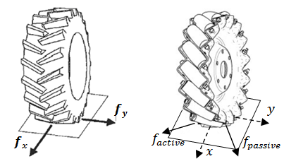
Figure 9. The most popular omnidirectional platforms in simulation, rendered by Dymola (rollers are not rendered for sake of effectiveness)

Note that the details of wheel geometry are not shown in the animation. The first platform is a simplified industrial forklift, it has four wheels, with rollers mounted at a angle (Mecanum wheels). I used lumped dynamic models. The vehicle body is represented by a point mass with inertia, and the load is represented by a simple point mass. Both the position and value of the masses, as well as vehicle dimensions are configurable. I also built a model of a three wheeled robot, with rollers. Its body is represented by a point mass with inertia.

Speed measurement feedback can be realized by any convenient method, however I propose an optical speed sensor mounted on the platform, described in[9]. The sensor measures true ground speed, and angular velocity, and works much like a conventional optical mouse. In the simulation the sensor is included by quantizing the simulated platform linear and angular speed values with a zero order hold, and adding random noise.

Braking is realized by simulated hydraulic disc brakes mounted on the driveshaft; a wheel can be either driven by a torque (motor), slowed or stalled by braking or let to roll freely.

The control loop works the following way: When the “driver” – or “autopilot” – pushes the brake pedal i.e. commanded brake force surpasses a limit, the brake assist gets activated and the value of , current linear velocity is stored. While braking, instantaneous wheel center velocities are calculated according to equation (4), based on the instantaneous platform velocity values and that are “measured” by an optical feedback unit. During the braking maneuver the controller continuously evaluates the error functions for each wheel. Based on the sign of the -th error function the actuator at the wheel lets the brake activate, – the brake force asserted by the “driver” gets applied – or inhibits braking – lets the wheel roll freely. For practical reasons, to avoid low speed drift, the brake assist is only active above a certain velocity threshold, below that it is switched off, and all the brakes are activated normally.

3.1. Idealized Experiment

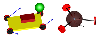
Figure 10. Braking in a straight line – snapshots, slowing from 10m/s

Figure 10 shows a demonstration of the brake assistant, with no external disturbances. The figure shows snapshots from an animation of an emergency braking trajectory at regular intervals. The upper part shows a run with the brake assist deactivated, the lower part shows the same experiment with the brake assist activated. Initial velocity is 10m/s. The difference between the two trajectories is obvious, with the brake assist activated, the vehicle does not swerve, but keeps its initial direction of movement.

Figure 11 shows linear and angular velocity components of the platform in body coordinates and the value of the function for each wheel vs. time. The brakes were engaged at 4s. A change in the direction of friction forces is well visible at 5s.

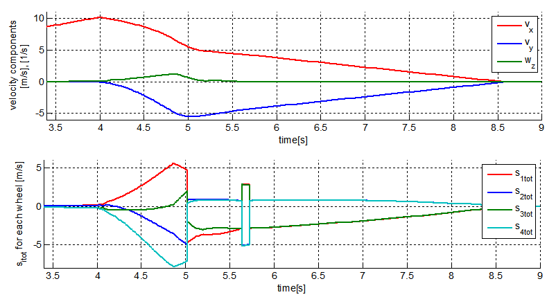Figure 11. Platform velocity components in body reference and function for a straight line braking maneuver. Mecanum platform, unassisted case

Figure 13 shows the same quantities for the same experiment, this time with the brake assist activated. It is worth noting that during the braking process the platform only has a velocity component in the x direction the y component and the angular velocity are negligible.

3.2. Disturbance Rejection and Practical Considerations

While in theory ideal sliding mode can be reached by applying infinite actuator frequency, in reality that is impossible to achieve. In practice actuator frequency needs to be sufficiently high compared to time constants of the controlled plant.

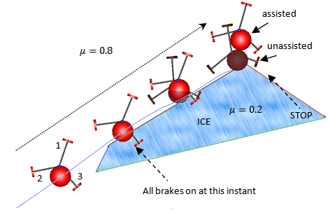Figure 12. Disturbance rejection: snapshots of braking on “ice”. Bright platform – assist on, dark platform – assist off

To model the effect of limited actuator frequency I quantized the update of feedback values and kept the velocity values constant for 10ms. Because of this the value of the function did not change, keeping the actuator state constant, limiting feedback speed.

To introduce unstructured disturbance I created a patch on the ground with a smaller friction coefficient and made the vehicle brake with some of its wheels on the “icy patch” and the others on regular ground. I also added some noise to the feedback. Noise is simulated by a uniform distribution centered around the real value with an adjustable percentage limit⁴. It can be set independently for the linear and the angular velocities. Also an offset can be incorporated in the signal.

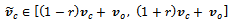(21)

where is the noisy linear velocity signal, is a percentage value, and is an offset. Similarly

(22)

where is the noisy angular velocity measurement p is a percent value and is an offset. Figure 12 shows overlaid snapshots of an assisted and non-assisted braking maneuver on an ice patch, with a noisy feedback signal, where The brighter colored platform had an active brake assist with a noisy feedback, the dark platform had no brake assist.

The experiment demonstrates that the controller tolerates the disturbances really well, as opposed to the unassisted case it does not swerve but keeps its orientation. As a disadvantage it can be noted that braking distance is a little longer in the assisted case, due to adaptation of brake forces to the lower friction on all wheels. Error and velocity signals are shown on Figure 14. Actuator signals are shown on Figure 15, for the three wheels in the order marked on Figure 13. The frequency at which the actuators work is well within the capabilities of hydraulic valves used in contemporary ABS systems.

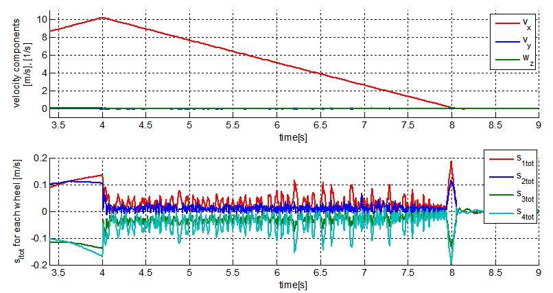Figure 13. Velocity components and values vs. time while braking from a straight 10m/s run. Mecanum platform, brake assist on

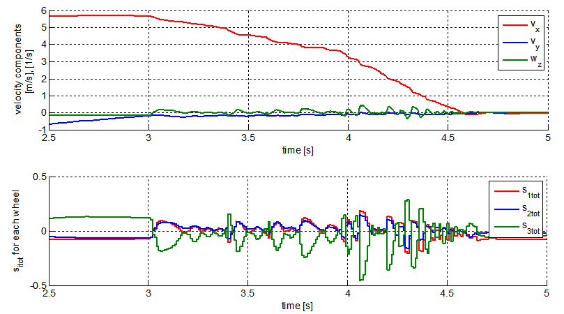Figure 14. Velocity components and error function for the ice patch experiment. Three wheel platform, assist on, leaving ice at 4s

4. Conclusions

In this article a brake assist controller was presented that is generally applicable for omnidirectional vehicles. The controller eliminates the swerving tendency that manifests during braking. The control law is created under the assumption that there are high uncertainties in the platform model, exact wheel characteristics and load distribution are deemed unknown. Also noise is assumed to be present in the velocity feedback and the friction coefficient of the ground. Due to these uncertainties and the nonlinear nature of the control problem sliding mode control was applied. The sliding manifold is constructed so that the velocity components of each wheel due to platform angular velocity and sideways linear velocity are driven to zero. The cross coupled nature of the general kinematic model ensures that this control approach stops the platform in finite time. The stability of the closed control loop is ensured by the passivity approach.

In the end of the article simulated experiments are presented, in which the two most popular omnidirectional platforms are tested, in the presence of disturbances. The controller was able to effectively stop the platforms, in a distance comparable to the unassisted case, but without swerving. The simulated platforms have dynamic properties, mass inertia, wheels with first order dynamics, but the controller does not use any knowledge about them.

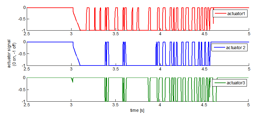Figure 15. Actuator signals at the wheels 1, 2 and 3. Brake is on when signal is 0, off when -1. Vehicle leaves ice at 4s

The simulations were carried out with a 10ms sampling time set for the feedback loop. As described in section 2.2 the controller equations contain mostly vector projection calculations, posing no real time challenge for contemporary embedded hardware, especially if look up tables are used for trigonometric functions.

Results in the dynamic simulation environment are promising, however further plans include testing the algorithm on a real platform to verify expected performance.

ACKNOWLEDGEMENTS

The author would like to thank Dr. László Vajta for inspiration and helpful suggestions, Dr. Tamás Juhász for his help with Modelica, and people at the IFF Fraunhofer Institute, Magdeburg, where some of the simulations were carried out.

Notes

1. www.airtrax.com, www.kuka-omnimove.com,[20], [21],[22]

2. The interested reader is referred to[8].

3. https://modelica.org

4. Uniform distribution might not be the best simulation of sensor noise, however my purpose here is to demonstrate disturbance rejection of the controller.