-
Paper Information
- Next Paper
- Previous Paper
- Paper Submission
-
Journal Information
- About This Journal
- Editorial Board
- Current Issue
- Archive
- Author Guidelines
- Contact Us
International Journal of Control Science and Engineering
p-ISSN: 2168-4952 e-ISSN: 2168-4960
2013; 3(1): 8-21
doi:10.5923/j.control.20130301.02
Robust Controller Design for an Electrostatic Micromechanical Actuator
 Abstract
 Reference
 Full-Text PDF
 Full-text HTML
1Department of Electrical and Computer Engineering, Cleveland State University, Cleveland, OH 44115, USA
2Nasa Glenn Research Center, Cleveland, OH 44135, USA
Correspondence to: Lili Dong, Department of Electrical and Computer Engineering, Cleveland State University, Cleveland, OH 44115, USA.
| Email: |  |
Copyright © 2012 Scientific & Academic Publishing. All Rights Reserved.
In this paper, a robust feedback controller is developed on an electrostatic micromechanical actuator to extend the travel range of it beyond pull-in limit. The actuator system is linearized at multiple operating points, and the controller is constructed based on the linearized model. Two kinds of controller designs are developed for set-point tracking of the actuator despite the presences of sensor noise and external disturbance. One of them is a regular fourth order Active Disturbance Rejection Controller (ADRC) and is able to achieve 97% of the maximum travel range. And the other one is a novel multi-loop controller with a second order ADRC in an inner loop and a PI controller in an outer loop. The multi-loop controller can achieve 99% of the maximum travel range. Transfer function representations of both controller designs are developed. The controllers are successfully applied and simulated on a parallel-plate electrostatic actuator model. The simulation results and frequency domain analyses verified the effectiveness of the controllers in extending the travel range of the actuator, in disturbance rejection, and in noise attenuation.
Keywords: Electrostatic Micromechanical Actuator, Active Disturbance Rejection Controller, Sensor Noise, Set-point tracking, Pull-in limit
Cite this paper: Lili Dong, Jason Edwards, Robust Controller Design for an Electrostatic Micromechanical Actuator, International Journal of Control Science and Engineering, Vol. 3 No. 1, 2013, pp. 8-21. doi: 10.5923/j.control.20130301.02.
Article Outline
1. Introduction
- Electrostatic actuation of micro-electro-mechanical systems (MEMS) makes use of the attractive electrostatic force between two charged capacitor plates to perform physical movements. With the advancement of MEMS technology, electrostatic (or micro-mechanical) actuators have been broadly used in micro-resonators, switches, micro-mirrors, accelerometers, and so on[1]. They are simple in structure, flexible in operation, and can be batch fabricated from standard semi-conductor materials such as silicon and poly-silicon[2]. The simplest electrostatic actuator has one degree of freedom and consists of one movable and one fixed capacitor plates in an electric field. When the movable plate is displaced from its original position, the capacitance formed between the two plates is changed. Therefore, one can change the displacement of the movable plate through a voltage control of the gap between both plates. However, as the gap is decreased to two thirds of the original gap, a pull-in (or snap-down) phenomenon will cause the instability of the system. As a result, the movable plate is dragged to the fixed plate, immediately reducing the gap to zero[1]. Thus extending the travelling range of the movable plate beyond the pull-in limit has been attractive to more and more researchers. In addition, the imperfections in fabrication and packaging technology introduce system uncertainties, external disturbance and noise to the actuator system. So a controller that can stabilize the actuator system and is robust against system uncertainties, disturbance, and noise is essential for improving the performance of electrostatic actuators. Since 1980’s, both open-loop and closed-loop controllers have been applied to electrostatic actuators. Open-loop controllers have the advantages of simple structure and easy implementation. Therefore the majority of MEMS actuators are driven in open-loop mode[2]. In order to overcome pull-in limit, the most straightforward open-loop solution is to design the gap so large that the actuator is stable over the desired operating range[3]. The drawback of this approach is that the maximum gap is determined by the fabrication technology and cannot be changed by the designer. Leverage bending[4] and strain stiffening[4] are another two approaches which are used to improve the dynamic behaviour of electrostatic actuators through structure design enhancements. It is shown in[4] that both approaches extend the travel distance of the actuator to about 60% of the full gap. In addition to the structural modifications for the mechanical part of MEMS actuators, alteration of the control voltages in the electrical part has been used. Introduction of complex actuating signals to the electrostatic actuator has resulted in so-called “pre-shaped control”[5], for which the dynamic model of the actuator is used to construct a pre-shaped input signal to improve the performance of it. The pre-shaped driving technique can extend the travel range of an electrostatic actuator to about 80% of its full gap. However, like other open-loop solutions, the pre-shaped control method is not robust against system uncertainties and external disturbance. The lack of accurate models, compounded by special requirements on the dynamic behaviour of actuators, has opened the possibility of closed-loop applications[5]. For closed-loop control strategies, utilizing a voltage source with a capacitor in series with the electrostatic actuator has proven successful[6, 7]. The technique shows stable operations of the actuator at 30%, 60%, and 90% of its full gap. The downside to this approach is that system uncertainties can degrade the control performance. Another disadvantage of it is that a large actuation voltage is required for the voltage source. This requirement significantly limits its feasibility. In[8, 9], a linear time-invariant (LTI) proportional gain controller is developed utilizing quantitative feedback theory (QFT). In the current literature, the LTI controller reported in[8, 9] is the only closed-loop controller that is implemented on a real MEMS actuator, and is able to extend the travelling range of it to 60% of the full gap. However a large loop gain of the LTI control system results in large noise amplification. Hence the controller cannot attenuate high-frequency input noises. More recently, nonlinear controls are applied to MEMS actuators[10]. In[11, 12], two robust nonlinear controllers are constructed based on input-to-state stabilization and back-stepping state feedback design respectively. Simulation results show that the nonlinear controllers can drive the actuator to reach full-gap traversal albeit with a large actuation voltage. But the usage of the controllers in[11, 12] is offset by their mathematical complexity and their lack of noise attenuation. In this paper, a linear, robust, closed-loop voltage control method is developed on a parallel-plate electrostatic actuator. The controller is based on an active disturbance rejection concept. The active disturbance rejection controller (ADRC) handles unknown system dynamics effectively by treating them as an unknown disturbance and cancelling them out in control law. In addition, it is robust against external disturbance and noise. A classic ADRC consists of an extended state observer (ESO), which is used to estimate internal dynamics and external disturbance, and a PD controller, which is used to drive the system output to a reference signal. It only has three tuning parameters that are controller and observer bandwidths and controller gain. The simple configuration and easy-to-tune feature make ADRC successful in multiple applications. The classic ADRC has ever been employed to MEMS gyroscopes[13], power systems[14], automobile systems[15], and web tensions regulation[16]. In this paper, we apply both classic ADRC and a novel multiple-loop ADRC to the electrostatic actuator respectively. For classic ADRC design, the displacement of the movable plate of an actuator is assumed available. For multiple-loop ADRC design, both displacement and charge outputs of the actuator are assumed measurable. The multi-loop design employs an ADRC for the inner loop to control the charge output, along with a PI controller in the outer loop to control the displacement output. Simulation results show that the classic ADRC design can drive the movable plate of an actuator to 97% of its full gap while the multi-loop design can achieve the traversal of 99% of the full gap. The multi-loop design also shows better noise attenuation capability than the classic one. Frequency-domain analyses proved the stability and robustness of the two designs against system uncertainties, disturbance, and noise.
2. Dynamic Modeling of MEMS Actuator
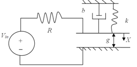
- An electro-mechanical model of a simple MEMS actuator with one degree of freedom is shown in Figure 1.
 | Figure 1. Micro-mechanical actuator model |
 | (1) |
2.1. Dynamic Modeling Using First Principles
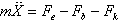
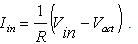
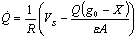
- The actuator in Figure 1 is operating in two energy domains, electrical and mechanical. As electrical charge (represented by Q) on the two plates builds up, the force of attraction grows, bringing the plates closer together. In order to keep the plates from touching each other there needs to be an equal and opposite force resisting this motion. This force is provided by the restoring spring force of a mechanical spring. In the mechanical domain, according to Newton’s 2nd law, we have
 | (2) |
 is the linear squeeze-film damping force, Fk=kX is the linear mechanical spring force and Fe=Q2/2εA is the nonlinear electrostatic force. Equation (2) can be rewritten as
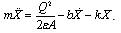 | (3) |
 | (4) |
 | (5) |
 , we have
  | (6) |
 | (7) |
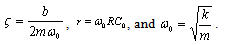
2.2. Equation Normalization
- For the simplicity of a controller design for the electrostatic actuator, equations (3) and (7) have to be normalized. The position of the upper plate relative to the lower plate (X), time (t), the charge (Q), and the source voltage (Vin) are normalized as follows.
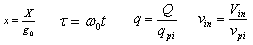 | (8) |
 | (9) |
 | (10) |
 | (11) |
 | (12) |
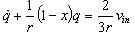
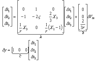
2.3. Model Linearization
- We choose the state variables of the normalized model of the actuator as x(t), q(t), and s(t), where s(t) is the velocity
 of the movable plate of the actuator. For small-signal linearization, the equilibrium values of the state variables, which are represented by Xeq, Qeq, and Seq, have to be determined. Then the nonlinear equation will be linearized around these equilibrium values. The state equations of the normalized actuator model are
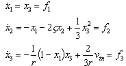 | (13) |
 | (14) |
 | (15) |
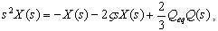
2.4. Transfer Function Representation of Linearized Model
- For the convenience of later frequency-domain analyses, a transfer function representation of the linearized electrostatic actuator model is developed. Conducting Laplace transform on (15) (assuming zero initial conditions) for the displacement output gives
 | (16) |
 | (17) |
 | (18) |
 | (19) |
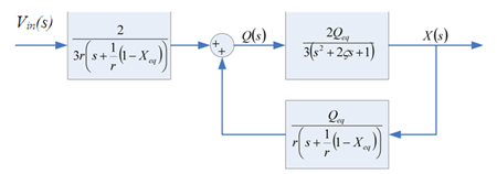 | Figure 2. Transfer function model of a MEMS actuator |
 | (20) |
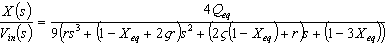
 | Figure 3. Simplified transfer function model |
 | (21) |
3. Controller Design
- In this section, two kinds of linear ADRC designs are presented. They are classic ADCRC and an original multi-loop ADRCs. The state space representations of the classic ADRC design are developed. Then the transfer function representations for both of the ADRC designs are derived for later frequency-domain analyses.
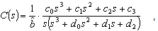
3.1. Classic ADRC Design
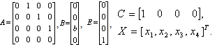
- For classic ADRC, all of the system parameters in (21) are assumed to be unknown. A fourth-order extended state observer (ESO) is developed to estimate both internal system states (including displacement, velocity, and charge) and external disturbance. Based on the accurate estimation of ESO, the classic ADRC is constructed to drive the actuator’s output to a desired displacement.
3.1.1. Introduction to Classic ADRC Design
- From (20) and (21), the electrostatic actuator can be modeled by a third-order differential equation as follows.
 | (22) |
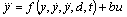
 , which will be denoted as f in the rest part of the paper, represents all of the other forces on the actuator plant excluding control effort, y(t) is equal to normalized displacement output x(t), d denotes external disturbance force, b is controller gain, and u is equal to Vin in (20). As we design the ADRC, the function f is assumed to be unknown and referred to as a generalized disturbance. We choose state variables as
  ,
,  ,
,  and
and  , among which x4 is an augmented state. Assuming
  and h is bounded within the interests, (22) can be represented by a state-space model as follows.
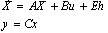 | (23) |
 | (24) |
 | (25) |
 | (26) |
 ,
,  and f. We assume that
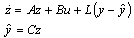
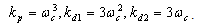
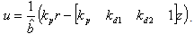
  is an approximate b. Then the control input to the actuator is
  | (27) |
 | (28) |
 | (29) |
 | (30) |
 .
.3.1.2. Transfer Function Representation of the Classic ADRC
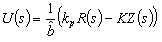
- Combing (27) and (29), we can rewrite the control input as
 | (27) |
 | (28) |
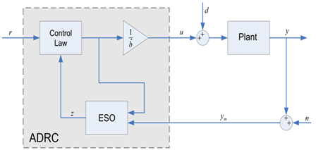 | Figure 4. Framework of classic ADRC |
 | (29) |
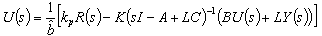 | (30) |
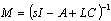 . Then (30) can be reorganized and simplified as
 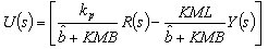 | (31) |
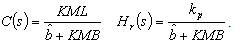 | (32) |
 | Figure 5. Block diagram of the classic ADRC control system |
 | (33) |
 | (34) |
 , and
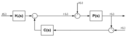
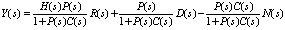
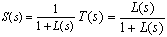
, and 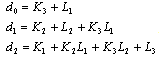 .As shown in Figure 3, the reference signal r and the measurement output y are treated independently by a pre-filter and ADRC. In addition, the configuration shown in Figure 5 allows for the derivations of traditionally defined sensitivity function (S), complementary sensitivity function (T), and other various closed loop transfer functions that are used for controller performance analyses to be conducted in the following section.
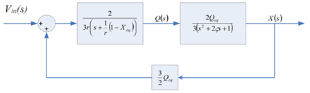
3.2. Multi-loop ADRC Design
- In this section, an original multi-loop control system is developed for the electrostatic actuator. The multi-loop control system consists of a standard ADRC in an inner loop and a traditional PI controller in an outer loop. The ADRC is used to control the charge output for the electrical part of the actuator while the PI controller is employed to control the displacement output for the mechanical part of the actuator. It would be demonstrated in the next section that adding an extra measured output (charge output) to the controller design can greatly reduces the effects of sensor noise and external disturbance on the actuator system.
3.2.1. Architecture of Multi-loop Control System
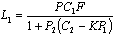
- We suppose the electrostatic actuator (as shown in Figure 3) can be divided into two sub-plants, which are P1 and P2, along with a positive feedback constant K. The two sub-plants and the feedback constant are defined as
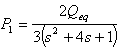 | (35) |
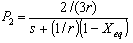 | (36) |
 | (37) |
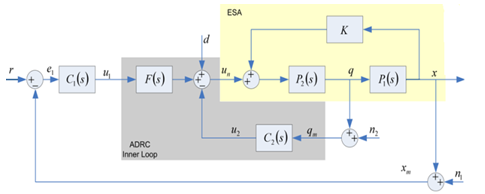 | Figure 6. Multi-loop control system |
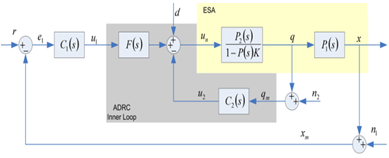 | Figure 7. Equivalent model of multi-loop control system |
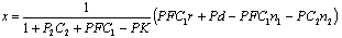 | (38) |
 | (39) |
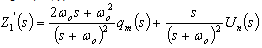
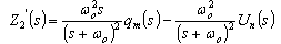
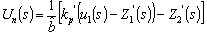
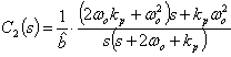
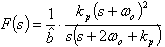
3.2.2. Inner Loop Design
- In the inner loop of the multi-loop control system (shown in Figure 6), the sub-plant P2(s) is a first-order system. Therefore an ADRC with a 2nd order ESO is applied in the inner loop. We choose the observer gain vector (L’) for the 2nd order ESO as L’=[2ωo, ωo2], where ωo is the observer bandwidth. Following the same equation development as we did for classic ADRC (in section 3.1), we will obtain the transfer function representation of the estimated charge output (Z1’(s)) as
 | (40) |
 | (41) |
 | (42) |
 . Substituting (40) and (41) into (42) yields
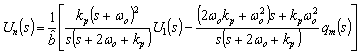 | (43) |
 | (44) |
 | (45) |
 | (46) |
3.2.3. Outer Loop Design
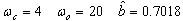
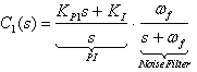
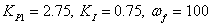
- In the outer loop of multi-loop control system, a PI controller that includes a first-order noise filter is used to control the displacement output of the sub-plant P1(s) of ESA. The PI controller is defined by (47), where Kp1 is a proportional gain, Kd1 is an integral gain, and ωf is the cut-off frequency of the noise filter.
 | (47) |
 | (48) |
4. Stability and Robustness Analyses
- In this section, we investigate the stability and the robustness against noise and disturbance for both classic ADRC and multi-loop control system designs.
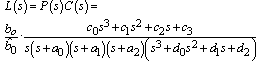
4.1. Loop Transmission and Sensitivity Functions for Classic ADRC Design
- In the frequency domain, the loop transmission function is a key tool in accessing the performance of a control system. For a classic ADRC design, the loop transmission function L(s) in Figure 5 is defined by
 | (49) |
 | (50) |
 | (51) |
 | (52) |
 | (53) |
 | (54) |
 | (55) |
4.2. Loop Transmission and Sensitivity Functions for Multi-loop Design
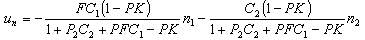
- From Figure 7, the effects of sensor noise on the control input (un) to the plant are represented by
 | (56) |
 | (57) |
 | (58) |
 | (59) |
 | (60) |
4.3. Stability Analyses
- The Bode diagrams of the loop transmission function L(jω) ((50)) for classic design are shown in Figure 8, where L05 represents the L(jω) for the desired travel range being 5% of the full gap. The plant for this travel range is denoted by P05. Similarly, L20, L33, L50, L75, and L95 represent the loop transmission functions for the desired travel ranges being 20%, 33%, 50%, 75% and 95% of the full gap. Note that the plant P33 is linearized at the pull-in displacement. In Figure8, three of the plants have unstable poles in the RHP (P50, P75, and P95), one has a pole at the origin (P33), and the other two are stable (P05, P20). The stability margins for the first design are listed in Table 1. The Bode diagrams of the loop transmission function ((57)) with respect to different displacements for multi-loop design are illustrated in Figure 9. Table 2 shows the stability margins for the multi-loop design. The bandwidth for multi-loop design is reduced but not significantly compared to classic ADRC design. Both classic ADRC and multi-loop designs have sufficiently large, positive stability margins which demonstrate the stability of these two designs.
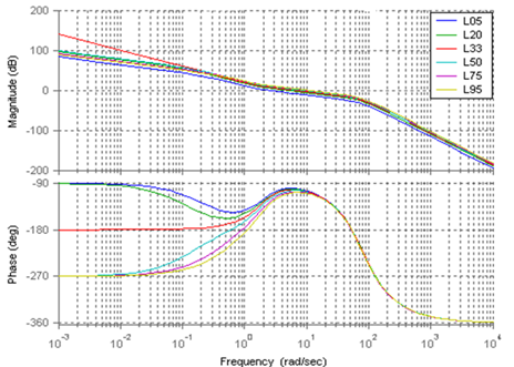 | Figure 8. Bode diagrams of the transmission function for classic ADRC design |
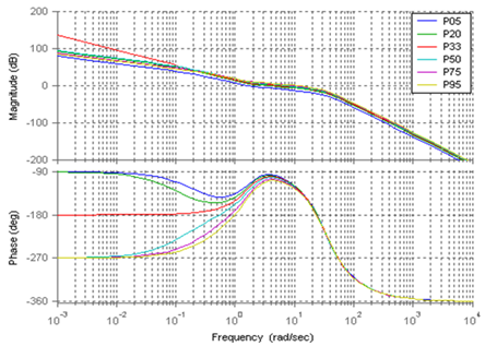 | Figure 9. Bode diagrams of the loop transmission function for multi-loop design |
|
4.4. Noise Attenuation
- For multi-loop control system, the transfer functions from two sensor noise sources (n1 and n2) to a single controller input (un) are given by (56). The Bode plots of these two transfer functions (in (56)) along with the Bode plot of the noise sensitivity function (54) for classic ADRC design are shown in Figure 10. In this figure, the multi-loop n1represents the Bode plot of the transfer function from noise source n1 to control input un, and multi-loop n2 represents the one from noise source n2 to control input un.
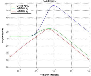 | Figure 10. Magnitude Frequency Responses of Controller Noise Transfer Functions for Both Multi-loop (with noise filter) and Classic ADRC Designs |
4.5. Disturbance Rejection
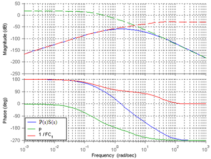
- Figure 11 shows the Bode diagrams of the input disturbance transfer function (55), along with the transfer function of an actuator model (P90), the inverse of the controller (or C-1 from (33)) and the loop transmission function (50) for classis ADRC design. From this figure, we can see that at low frequencies, P(s)S(s) (in (55)) behaves like C-1, while at high frequencies, it behaves like plant model P90. Thus if controller C has high gain at low frequencies, C-1 will attenuate low frequency disturbance. It’s also shown that when the magnitude of L(s) is small, the controller has no control over high frequency disturbance. Then the disturbance will follow the high frequency behaviour of the actuator plant. Figure 12 shows the bode diagrams the input disturbance transfer function (60), the transfer function of the actuator plant (P90), and the inverse of F(s)C1(s) in Figure 6. From this figure, we can see that the inverse of F(s)C1(s) plays a dominate role in input disturbance rejection at low frequency. However, at high frequency part, the disturbance rejection is solely dependent on the actuator plant. The electrostatic actuator has built-in disturbance rejection capabilities due to its low system gain. However, both classic ADRC design and multi-loop control system demonstrate excellent disturbance rejection capabilities at low frequency part. In summary, the multi-loop controller is equally good as classic ADRC when it comes to stabilizing the actuator system and disturbance rejection. However, the multi-loop controller shows much better noise attenuation capability than classic ADRC design.
 | Figure 11. Bode diagrams of input disturbance function, actuator model, the inverse of controller, and loop transmission function for classic ADRC design |
 | Figure 12. Bode diagrams of input disturbance transfer function, actuator model, and inverse of F(s)C1(s) |
5. Simulation Results
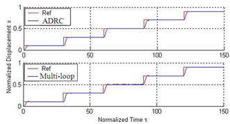
- During the simulation, the senor noise in Figure13 is added to the control systems shown in Figure5 (as N) and Figure 6 (as n1 and n2) respectively. Both the classic ADRC design and the multi-loop control system are simulated on the normalized model of the electrostatic actuator, whose parameter values are given in Table 4 of Appendix. Figure 14 and Figure 15 show the step responses of the two kinds of control designs to the references of 10% and 99% of the full gap respectively. In both figures, blue line represents reference signal. From Figure 14, we can see that the rise time of the classic ADRC is much smaller than the one for the multi-loop controller at small displacement. However, the step response of the multi-loop control system has zero overshoot while the classic ADRC design exhibits overshoot. Figure 15 demonstrates that only the multi-loop design can achieve 99% of full gap traversal. The overshoot in the step response of the classic ADRC system will result in the “snap down” between the two plates of the actuator and cause the failure of operation. Figure 16 shows the control signals for both designs in the presence of sensor noises. It is clear to see that the multi-loop controller is a better choice in minimizing the effects of sensor noise than the classic ADRC design. Figure 17 shows the displacement outputs for the two designs with a step disturbance at t=15s. The figure demonstrates the robustness of the two designs with a travel range of 97% of initial gap in the presence of the disturbance. From Figure 17, we can see that the multi-loop design has much smaller overshoot than the classic ADRC when a step disturbance is added to the system. Figure 18 compares the tracking performances of the two ADRC designs. In Figure18, the actuator is commanded to track several desired travel ranges which are set to 10%, 30%, 50%, 70% and 90% of the full gap. Both designs have shown excellent tracking performances. The simulation results demonstrate the better performance of multi-loop control system than classic ADRC controlled system in noise attenuation and disturbance rejection. However, the classic ADRC has smaller rise time than the multi-loop design.
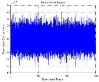 | Figure 13. Normalized sensor noise |
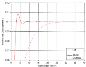 | Figure 14. Step responses of two control designs at 10% of full gap |
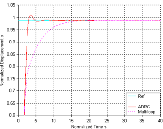 | Figure 15. Step responses of two controller designs at 99% of full gap |
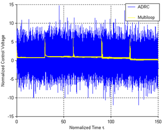 | Figure 16. Controller signals for the two designs with sensor noise |
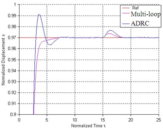 | Figure 17. Displacement outputs of two designs with step input disturbances at t=15s |
 | Figure 18. Displacement outputs of two designs |
6. Conclusions
- The research presented in the paper aims to provide a robust feedback controller that could greatly increase the operating range of an electrostatic actuator and to stabilize the actuator over the entire operating range. This controller would have to overcome the pull-in phenomenon inherent in the actuator. It also has to cope with sensor noise and external disturbance. And most importantly, the controller needs to be simple enough to implement on a MEMS device where silicon area is at a premium. The contribution of this research is that two forms of linear ADRC designs are developed that provide nearly full gap traversal for the actuator despite the presences of sensor noise and disturbances. Both controller designs have successfully addressed all the control problems state above. In addition to the effectiveness of these controllers they only have three tuning parameters, and hence are simple enough for practical implementation.The classic ADRC design could drive the electrostatic actuator to travel 97% of its full gap. But this design is sensitive to sensor noise compared to multi-loop design. The multi-loop controller shows great promise in controlling the electrostatic actuator to 100% travel range, while keeping the effects of sensor noise to a minimum. This design should be considered as a design of the future since current technology makes it difficult to obtain two sensed outputs, but it does serve as a benchmark for what is possible with feedback control. As the complexity of MEMS devices increases, the demand for high performance control will also rise, making this design highly practical in the near future.
APPENDIX
|
|
References
| [1] | S.D. Senturia, Microsystem Design, Kluwer Academic Publishers, Norwell, MA, 2001. |
| [2] | Kovacs G. T. A. 1998, Micro-machined Transducers Sourcebook, McGraw-Hill, New York. |
| [3] | J. Seeger, “Charge control of parallel-plate, electrostatic actuators and the tip-in instability,” Journal of Micro-electro-mechanical Systems, vol. 12, no. 5, pp. 656-671, Oct. 2003. |
| [4] | E. S. Hung and S. D. Senturia, “Extending the travel range of analog-tuned electrostatic actuators,” Journal of Micro-electro-mechanical Systems, vol. 8, no. 4, pp. 497-505, Dec. 1999. |
| [5] | B. Borovic, “Open-loop versus closed-loop control of MEMS devices: choices and issues,” Journal of Micromechanics and Micro-engineering, vol. 15, no.10, pp. 1917-1924, Jul. 2005. |
| [6] | J. Seeger and S. Crary, “Stabilization of electro-statically actuated mechanical devices,” IEEE International Conference on Solid-State Sensors and Actuators, pp. 1133-1136, Jun. 1997. |
| [7] | E. Chan and R. Dutton, “Electrostatic micromechanical actuator with extended range of travel,” Journal of Micro-electro-mechanical Systems, vol. 9, no. 3, pp. 321-328, Sep. 2000. |
| [8] | S. Zhang, C. Zhu, J. K. O. Sin, and P. K. T. Mok, “A novel ultrathin elevated channel low-temperature poly-Si TFT,” IEEE Electron Device Lett., vol. 20, pp. 569–571, Nov. 1999. |
| [9] | M. Wegmuller, J. P. von der Weid, P. Oberson, and N. Gisin, “High resolution fiber distributed measurements with coherent OFDR,” in Proc. ECOC’00, 2000, paper 11.3.4, p. 109. |
| [10] | G. Zhu, J. Levine, and L. Praly, “Improving the performance of an electrostatically actuated MEMS by nonlinear control: some advances and comparisons,” in Proc. of the 44th IEEE Conference on Decision and Control, pp. 7534-7539, Dec. 2005. |
| [11] | G. Zhu, J. Levine, and L. Praly, “On the differential flatness and control of electro-statically actuated MEMS,” in Proc. of 2005 American Control Conference, Portland, Oregon, pp. 2493-2498, June 2005. |
| [12] | G. Zhu, J. Penet, and L. Saydy, “Robust control of an electro-statically actuated MEMS in the presence of parasitics and parametric uncertainty,” in Proc. of the 2006 American Control Conference, pp. 1233-1238, Jun. 2006. |
| [13] | L. Dong, D. Avanesian, “Drive-mode Control for Vibrational MEMS Gyroscopes”, IEEE Transactions on Industrial Electronics, vol. 56, no. 4, pp. 956-963, Apr. 2009. |
| [14] | L. Dong, Q. Zheng, Z. Gao, “On Control System Design for the Conventional Mode of Operation of Vibrational Gyroscopes”, IEEE Sensors Journal, vol. 8, no. 11, pp. 1871-1878, Nov. 2008. |
| [15] | L. Dong, Y. Zhang, Z. Gao, “A Robust Decentralized Load Frequency Controller for Interconnected Power Systems”, ISA Transactions, vol. 51, no. 3, pp. 410-419, May 2012. |
| [16] | L. Dong, P. Kandula, Z. Gao, D. Wang, “A Novel Controller Design for Electric Power Assist Steering Systems”, Journal of Intelligent Control and Systems, vol. 15, no. 1, pp. 18-24, Mar. 2010. |
| [17] | Y. Hou, Z. Gao, F. Jiang, and B. Boulter, “Active disturbance rejection control for web tension regulation,” in Proc. of the 40th IEEE Conference on Decision and Control, vol. 5, pp. 4974-4979, Orlando, Florida, USA, Dec. 4-7, 2001. |
| [18] | Z. Gao, “Scaling and bandwidth-parameterization based controller tuning”, in Proc. of American Control Conference, Denver, CO, June 2003, vol. 6, pp. 4989 - 4996. |