1. Introduction

The growing attention has been paid to a parking assistance system (PAS) to provide more safety and convenience to a driver. The PASallows the driver to park a car without manual steering control and has been commercializedrecently by many automakers[1]. Furthermore, the advanced parking assistance system (APAS) (or called self-parking), which makes a vehicle parked autonomously, has been developed[2, 3].For instance, autonomous driving including autonomous valet parking (AVP) was demonstrated in the Urban Challengein 2007, which is an autonomous vehicle competition[4, 5]. Whereas it succeeded in showing the feasibility of autonomous drivingwith many additional sensors such as radars, lidars, cameras, and ultrasonic sensors to recognize lane, obstacles, and a parking lot, it is interesting to remark that the detection range to identify an available parking lot in a public parking structure is still limited.

Another approach is to develop an intelligent parking infrastructure whichprovides usefully driving information such as position of the vehicle, obstacles and location of anavailable parking space to either a driver or a vehicle wirelessly via vehicle to infrastructure (V2I) communication. Since a parking guidance system to identify an optimal parking lot and guide the route to the driver has been already developed[6], the development of the intelligent parking infrastructure is feasible if the positions of all vehicles in the parking structure can be measured or estimated.

One possible approach to obtain this information is to use a set of infrastructure sensors such as lidars and cameras, which are implemented in the parking structure, not on the vehicle[7]. That is,the infrastructure sensors detect all vehicles within their detection range, and positions of vehicles are estimated by combining all measurements of sensors and location of sensors centrally in an intelligent parking server.

In this paper, a semi-autonomous valet parking (SAVP) system with the cooperation of the intelligent parking infrastructure is considered under the assumption that a driver is in a vehicle and the velocity is controlled manually. Only steering control is performed automatically for forward driving to a parking lot and backward parking maneuvers. Furthermore, it is assumed that an optimal parking lot is identified and the corresponding route, i.e., a set of waypoints, is planned by the intelligent parking server, and the corresponding information is sent to the vehicle via V2I communication.

Among many challenging problems for SAVP in the area of perception, planning, communication, and control, a lateral control problem is only focused in this paper. More specifically speaking, the challenging control problems to be solved in this paper are summarized as follows:

•Both measurement noise (especially in position and heading angle) and model uncertainty are considered.

•Various driving maneuvers (e.g., forward driving, temporary stop, and backward parking) need to be conducted in a unified framework of lateral control.

•The driving performance should reflect the behavior of a human driver. Thus, the movement of steering is slow enough to satisfy kinematic constraints of a steering actuator.

2. Driving Scenario and Hardware

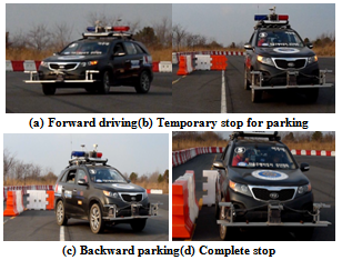
As shown in Fig. 1, it is assumed that the driving scenario for SAVP includes a series of driving maneuvers, i.e., forward driving on a straight and curved road (see a waypoint A to B in Fig. 1), temporary stop (at B in the figure), backward parallel parking (B to C in the figure), and complete stop at the waypoint C. Moreover, it is assumed that an available parking location is determined by an SAVP server which monitors all vehicles in a dedicated intelligent parking infrastructure. Then, the corresponding waypoints (refer to the circles in Fig. 1) are delivered to the vehicle controller via V2I communications.

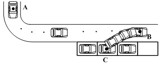Figure 1. Driving Scenario for SAVP

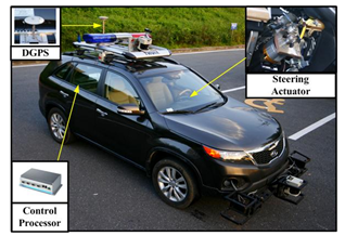Figure 2. Hardware Layout of Test Vehicle

To conduct the given driving maneuvers for SAVP, a test vehicle shown in Fig. 2 has the following capabilities:

•The steering wheel angle can be controlled by external commands determined from the vehicle controller. In fact, it is feasible if a motor drive power steering system (MDPS) which is already commercialized is available.

•Both position and heading angle of the vehicle with measurement noise are provided. It is noted that a DGPS is used for experimental validation of the proposed lateral controller as shown in Fig.2 although it will be replaced by infrastructure sensors in the near future.

•There is an electronic control unit (ECU) or processor to compute a steering angle command based on information via V2I communications.

• Gear engagement and wheel speed are measured by in-vehicle sensors and the information is sent to ECU via controller area network (CAN).

3. Lateral Control

The lateral controller to provide the desired steering wheel angle for SAVP needs both trajectory for different driving maneuvers and control laws. A kinematic vehicle model subject to kinematic constraints of the steering actuator is proposed and the model-based nonlinear control technique is applied for the controller design.

3.1. Trajectory Generation

To perform different driving maneuvers such as forward driving and backward parallel parkingas illustrated in Fig. 1, the corresponding trajectory is necessary for the lateral controller. Three approaches for the trajectory generation have been found mainly in the literature: a combination of lines and circles[8, 9], curve fitting[10], and clothoids[11]. In this section, both the combination of circles and curve fitting techniques are used for trajectory generation.

In the case of forward driving, the trajectory generation is interpreted as curve interpolation between two given waypoints. Suppose two waypoints are given as p₀ (or a point A) and p₃ (or a point B) as seen in Fig. 3. Ifa cubic Bezier curve interpolation approach is appliedwith two additional control points, p₁ and p₂, the trajectory for the forward driving isdetermined as follows:

(1)

where is the desired trajectory(or a set of reference points) between two waypoints with respect to a local coordinate originated at p₀, is equally spacing for , and the vectors a, b, and c are defined as

The shape and smoothness of the trajectory in (1) depends on the selection of two control point points(see p₁ and p₂ in Fig. 3). The control points are written in the coordinate from as follows:

(2)

wherel is a constant which determines the smoothness of trajectory,ψis the yaw angle of the vehicle, and is the angle between p₃ and next waypoint. However, it is noted that is a predefined angle when the vehicle reaches the waypoint where the parking maneuver begins (refer to a waypoint B in Fig. 3).

For the backward parallel parking, one of the simplest trajectory generation techniques is to use two circles based on Ackermann steering geometry of the vehicle[6]. When the vehicle arrives at an available parking location, i.e., near a waypoint Bin Fig. 3, it is assumed that a parking end point, i.e., a waypoint C in Fig. 3, is given via V2I communication.To generate two circles for parallel parking, an intersection point of two circles, Q in Fig. 3, is first calculated under the assumption that two circles with the same radius are used. Since a circle is uniquely determined when two points on the circle are known, a center and radius of the circle passing a current position near a waypoint B and Q can be determined as follows:

Since the center of the second circle, T, can be obtained similarly, the trajectory for the parallel parking can be summarized as follows:

(3)

where the subscript dstands for thedesired trajectory, and thesubscripts x and y are the positions with respect to x and y directions respectively.

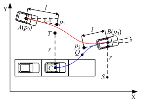Figure 3. TrajectoryGeneration for SAVP

3.2. Vehicle Model

A bicycle model has been used widely for design of the lateral controller for highway driving[12]. It is assumed that all system parameters of tire stiffness are known and all wheel angles are small. However, a large amount of wheel angle is generated for parking and it is not easy to identify the system parameters for various types of vehicles.

For the SAVP, the vehicle is driving at low speed and thus sideslip angle is neglected in this study. Thus, the kinematic model can be used for both driving and parallel parking.The equation of motion is written as follows[13, 14]:

(4)

where x and y are the longitudinal and lateral positions of the vehicle, v is the vehicle speed, and δis the steering angle. In addition, the subscript i represents the driving maneuver, i.e., f is forward driving and b is backward driving. It is noted that the effective length of wheelbase, L_i, instead of the length of wheelbase (L), is used with respect to driving maneuver. Furthermore, the kinematic constraints of a steering actuator are considered and they are written as

(5)

where δ_max, ω_max are the maximum steering angle and angular velocity respectively.

Suppose a set of parameters in (4) and (5) are given as

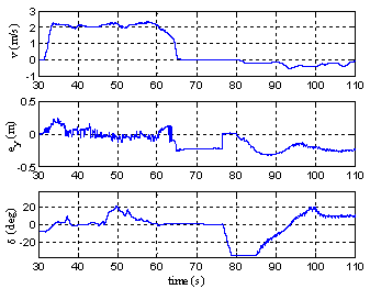
The time responses of the vehicle model in (4) and (5) are compared with experimental data using a test vehicle shown in Fig. 2. The vehicle is driven forward manually from 0 to about 75 second, stopped temporarily to changegear engagement for backward driving, and driven backward from about 78 to 110 second (see the first plot in Fig. 4). The corresponding steering angle is shown in the second plot of Fig. 4. Around 78 second, the maximum steering angle is required for backward parking and the maximum angular velocity of the steering angle is shown at that time. The angular velocity is approximated by use of difference of the steering angle of five samples as follows:

Where T is a sampling time.

When the same velocity and steering angle satisfying the constraints in (5) are assigned, it is shown in the fourth and fifth plots of Fig. 4 that both responses of forward driving and backward parking are quite similar with the maximum error deviation of 0.11(rad) and 0.01(rad/s) in terms of the yaw angle and rate respectively

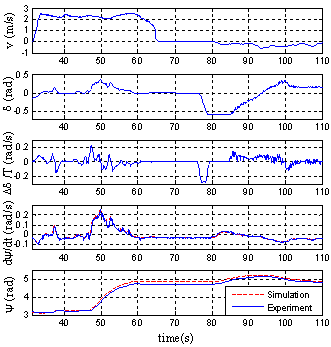Figure 4. Comparisonbetween Vehicle Model and ExperimentalData

3.3. Lateral Control Law

A model-based nonlinear control technique called dynamic surface control is applied to design alateral controllerat most of speed range[14, 15].First, the error surface is defined as follows (see also in Fig. 5)[14]:

(6)

where the lateral error e_y is defined as

(7)

the shortest distance from the current position to the desired trajectory, e_d, is calculated as

Where k^* is obtained iteratively by

andP_d comes from (1) for forward driving and (3) backward parking respectively. Furthermore, the sign of the lateral error in (7) is defined as follows:

Where [x_pdy_pd]^T is the preview point and m_i is a constant but two different values are assigned for forward driving and backward parking. When the vehicle is placed as in Fig. 5, c is negative and the lateral error in (7) becomes positive. Then, the positive (or counterclockwise) steering angle command will be determined by the lateral control law which will be discussed later. Furthermore, d_i and ψ_d in (6) are defined as

It is noted that the preview control idea is incorporated with DSC by considering both d_i andψ_d in (6)[8].

After differentiating S_i in (6) and combining it with (4), the time derivative of S_i is

(8)

To make S_i go to zero, let where K_i is acontroller gain. Then the desired steering angle is obtained as

(9)

(10)

Next, two possible cases which may make the control law in (10) violate the actuator constraints in (5) are considered. First, the desired steering angle in (10) can be changed rapidly due to the assignment of a large controller gain K_i or inclusion of measurement noise. Then the actual steering angle cannot follow the desired steering angle. To solve this problem, the lateral controller is redesigned by introducing a first order low-pass filter. That is, if the desired steering wheel is calculated after passing through as follows:

(11)

the desired steering angle is determined as

(12)

It is remarked that in (9) rather thanδ_des in (10) is filtered and it allows us to analyze the stability more easily and clearly[15].

For the second case, since the velocity is controlled manually by a driver, it can be very low or even zero. In this case, the desired steering angle in (10) becomes greater than δ_max, thus resulting in saturation of the actuator regardless of the lateral error or S_i in (6). Thus, two control laws are switched depending on velocity, i.e., a proportional controller is used when the velocity is very low. Otherwise, the lateral control law in (12) is used. Finally, the modified lateral control law is summarized as follows:

(13)

whereK_pi is a proportional controller gain and εis a velocity threshold.

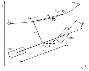Figure 5. Definitions of Lateral Error and Heading Angle Error

4. Validation Results

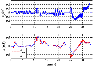
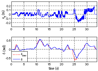
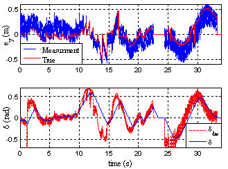
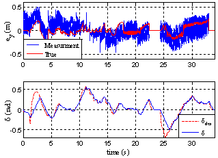
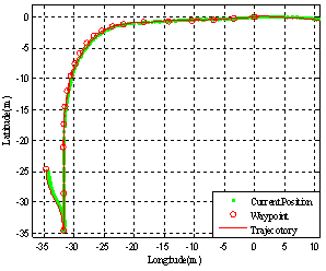
Suppose 21 waypoints are given as shown in Fig 6. The forward driving is required from the first to 20^th waypoint (A to B in the figure) and the backward parallel parking is asked from 20^th to 21^st waypoint (B to C in the figure). The proposed lateral controller is validated via a vehicle simulator called CarSim[16] and field tests using a test vehicle shown in Fig. 2.

First, the tracking performance of the lateral control law in (13) is validated via simulations with considerations of measurement noise and kinematic constraints of a steering actuator. Before evaluating the performance, it is shown in Fig 6 that trajectory for forward driving and backward parallel parking is generated appropriately. When measurement noise of position and yaw angle is not considered, the performance of the lateral controller in (10) is shown in Fig. 6 and 7. It is validated in Fig. 7 that two different driving maneuvers can be conducted by the single lateral controller with the maximum lateral error deviation of about 0.2 (m) (see the top plot in Fig. 7).

However, it is shown in the bottom plot of Fig 7 that the steering angle does not track the desired steering angle sometimes due to the kinematic constraint of the steering angular velocity. If the control law in (13) is used, it is shown in Fig. 8 that the desired steering angle does not violate the kinematic constraints much less than one in (10) without any performance degradation in the term of lateral error.

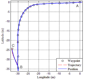Figure 6. Waypoint, Trajectory, and Position of Vehicle

Figure 7. Time Responses of Lateral Error and Steering Angle without Consideration of Noise

Suppose measurement noise of position and yaw angle is considered with variation of 0.2 (m) and 0.5 (deg) respectively. While the performance of the lateral controller in (10) is degraded with the maximum lateral error of about 0.5 (m) as shown in Fig. 9, one of the redesigned controller in (13) is not much in the presence of measurement noise and the kinematic constraints of the steering actuator (refer to Fig. 10). Fig. 11 shows the snapshot of forward following in the CarSim vehicle simulator.

Figure 8. Time Responses of Lateral Error and Steering Angle of the Modified Lateral Controller

Figure 9. Time Responses of Lateral Error and Steering Angle with Consideration of Measurement Noise

Figure 10. Time Responses of Lateral Error and Steering Angle of the Modified Lateral Controller

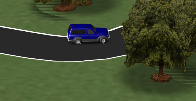Figure 11. Snapshot of Vehicle Simulation for Forward Driving

The proposed lateral controller is implemented in a real vehicle as shown in Fig. 2 and its performance is evaluated via field driving tests. For the given 21 waypoints (see circle marks in Fig. 12), it is shown that the vehicle follows the desired trajectory with a maximum lateral error deviation of about 0.3 (m)(see also the second plot in Fig. 13).Furthermore, the corresponding time responses of the lateral controller are shown in Fig. 13. It is shown that the vehicle arrives at 20^th waypoint at about 65 second and waits until the gear is shifted to backward. Then, the parallel parking maneuver begins at about 78 second. Finally, snapshots of forward driving, temporary stop, and backward parallel parking are shown in Fig. 14.

Figure 12. Position of Lateral Controller in Field Test

Figure 13. Time Responses of Lateral Controller in Field Test

Figure 14. Snapshots of Field Test

5. Conclusions

The lateral vehicle control algorithmbased on the vehicle model with kinematic constraints of the steering actuator was proposed. It was incorporated with the preview control, switching of multiple controllers, and filtering of the steering command to compensate for performance degradation due to measurement noise and manual control of velocity.Finally, it was validated via simulations and field tests that the proposed controller could be applied to conduct two different driving maneuvers,i.e., forward driving and parallel backward parking.

In the near future, it is necessary to consider more various parking maneuvers such as perpendicular and/or multi-step parking, forward parking, and effect of time delay and packet loss when V2I communication is used.

ACKNOWLEDGEMENTS

This research was supported by the Industrial Strategic Technology Development Program (10035250, Development of Spatial Awareness and Autonomous Driving Technology for Automatic Valet Parking) funded by the Ministry of Knowledge Economy (MKE, Korea).