1. Introduction

Hybrid dynamic systems constitute a particular class of dynamic systems in which some elements (called switching components) or phenomena evolve much faster than the time scale at which the system behaviour needs to be analysed[16]. Such systems, also called switched systems, are widespread in physical and engineering fields (hydraulic systems with valves, electrical systems containing diodes, relays or transistors,…, mechanical systems with clutches or collisions...). In this present work, I investigate the observability issue for controlled switching linear systems modelled by bond graph. My obtained results present a graphical method based on an energy concept.

Observability is a fundamental concept in modern control theory of systems, has been extensively studied both in the continuous and in discrete domains. More recently various researchers have approached the study of observability for hybrid systems[2, 14, 15, 18, 19].

Ezzine and Haddad[12] first studied the one-period controllability and observability for periodically switched systems, some sufficient and necessary conditions were established. Then, Xie and Zheng[6] introduced the multiple-period controllability and observability concepts naturally extended from the one-period ones, necessary, and sufficient criteria were derived. It was also pointed out that controllability can be realized in n periods at most, where n is the state dimension. As to arbitrarily switched linear systems, Sun and Zheng[21] first gave a sufficient condition and a necessary condition for controllability and proved that the necessary condition is also sufficient for three-dimensional systems with only two subsystems. Following the work in[21] and[22] extended the result to three-dimensional systems with arbitrary number of subsystems. Then, necessary and sufficient geometric type criteria for controllability and observability were derived in[22] and[7]. Vidal and al.[18] considered autonomous switching systems and proposed a definition of observability based on the concept of indistinguishability of continuous initial states and discrete state evolutions from the outputs in free evolution. Incremental observability was introduced in[2] for the Class of Piecewise Affine (PWA) systems. Incremental observability implies that different initial states always give different outputs independently of the applied input. In[1], a methodology was presented for the design of dynamic observers of hybrid systems that reconstructs the discrete state and the continuous state from the knowledge of the continuous and discrete outputs. In[10], the definitions of observability of[19] and the results of[1] on the design of an observer for deterministic hybrid systems are extended to discrete-time stochastic linear autonomous hybrid systems.

In order to obtain a more realistic model for the analysis of system properties, the concept of structural property has been introduced in[5], is true for almost all values of the parameters. This framework is consistent with physical reality in the sense that system parameter values are never exactly known, with an exception for zero values that express the absence of interactions or connections.

The elements of a structural matrix[A] are either fixed at zero or indeterminate values that are assumed to be independent of one another. Hence it is desirable to investigate system properties that are only determined by the structure of the system and not by the parameter numerical values. A useful tool for this purpose is the bond graph approach, which has received a great deal of attention in the last decade[5, 17]. This approach has been used for the analysis of structural properties of linear systems[3, 4, 9].

This paper is organized as follows: The second section, formulates the Controlled Switching Linear Systems (CSLS) observability. Section three recalls some background about bond graph modelling of hybrid systems with ideal switches. In section four the structural observability of these systems is discussed using bond graph model. Graphical conditions and procedures are also proposed. Finally, a simple example which illustrates the previous results is discussed.

2. Observability of Controlled Switching Linear Systems

Consider a controlled switching linear systems[23], described by

(1)

Where is the state variable, is the input variable, and is the output variable. is a piecewise constant switching function and the hybrid state.

If we consider this system in a particular mode i, the equation (1) can be written as :

(2)

With , , , and q the number of mode.

Remark 1 System (2) can be considered as a linear time invariant system (LTI).

Assumptions 1

1) We suppose that , and matrices are constant on ,where , and constant is an arbitrarily small and independent of mode . For instance, suppose that the dynamics in (1) are given by over the finite time interval . At time the dynamic in interval is given by .

2) We assume that the state vector does not jump discontinuously at .

Under these assumptions, the observability of (1) was defined:

Definition 1[22] The CSLS (1) is observable, if there exist a time and a switching path , such that initial state can be determined by the corresponding system input and the system output , .

2.1. An Algebraic Sufficient Condition

In order to investigate observability of (1), the following zero input system is considered.

(3)

It is obvious that the observability of (1) is equivalent to that of (3).

The observability combined matrix [9] of system (1) is given by equation (4),

(4)

where

is the observability matrix of the mode.

Theorem 1[9] The CSLS (1) is observable, if .

Remark 2 From this theorem, we can deduce that:

1) The system (1) can be observable, if there is only one observable sub-system (mode).

2) However, it is possible that no sub-system is observable but that the system (1) is observable.

2.2. A necessary and Sufficient Algebraic Condition

References[9] and[22] define the subspace sequence

, and

(5)

Theorem 2[22]System (1) is observable, if and only if .

This theorem is a geometric criterion, thus, it is easy to transform it into algebraic form.

Definition 2The joint observability matrix of system (1) is defined as :

(6)

With .

Theorem 3[9]System (1) is observable, if and only if .

Proof.For , we have :

For , we have :

In a similar way one finds :

However and , then

Of another share, we have :

With , ,

and

Then .

We exposed algebraic and geometric criteria of analysis of the properties of observability of CSLS. The next section is devoted to the graphic interpretation of these results by using the Bond graph approach.

3. Bond Graph Approach

The bond graph structure junction contains informations on the type of the elements constituting the system, and how they are interconnected, whatever the numerical values of parameters. The structure junction of a switching bond graph can be represented by Figure 1. Five fields model the components behaviour, four fields that belong to the standard bond graph formalism; - source field which produces energy, - detector field; - R field which dissipates it, - I and C field which can store it, - and the Sw field that is added for switching components.

Figure 1 represents the block diagram that is deduced from the causal bond graph.

The following key variables are used :

- the state vector x(t)is composed of the energy variables on the bond connected to an element in integral causality (the momenta on I elements and charges on C elements), and the complementary state vector z(t)is composed of power variables (the efforts eon Celements and flows f on I elements);

- and represent the variables going out of and into the R field;

- the vector u(t)is composed of the sources;

- is composed of the zero valued variables imposed by the switches in this configuration;

- is composed of the complementary variables in the switches;

- the vector y(t) is composed of the continuous outputs.

Figure 1. Structure junction

Assumptions 2

To take into account the absence of discontinuities (Assumption 1), we suppose that there are no elements in derivative causality in the bond graph model in integral causality, before and after commutation.

Using the structure junction, the following equation is given[11] :

(7)

. is a positive matrix. Let assume that is an invertible positive matrix. Then the second row leads to

.

The third line of (7) gives :

(8)

Then substituting also in the first line of (7) gives :

(9)

The output vector is given by :

(10)

When the elements of commutations are in the chosen configuration (mode i for example), then .

(11)

where , ,

, ,

and .

Therefore, for N switches and by considering, we have modes :

(12)

4. Structural Observability

The bond graph concept is an alternate representation of physical systems. Some recent works permit to highlight structural properties of these systems[4]and[3]. In[4], the structural observability property is studied using simple causal manipulations on the bond graph model. It is shown that the structural rank concept is somewhat different for bond graph models because it is more precise than for other representations. Our objective is to extend these properties to CSLS systems.

In the following we note that:

-BG: acausal (without causality) bond graph model,

-BGI: bond graph model when the preferential integral causality is affected,

-BGD: bond graph model when the preferential derivative causality is affected,

- : the number of elements in integral causality in BGD_i. i indicate the mode i.

- : the number of elements remaining in integral causality in BGD_i, when a dualization of the maximum number of continuous output y and discrete output is applied (in order to eliminate elements in integral causalities).

To study structural observability of CSLS modelled by bond graph, graphical methods are proposed in the form of two sufficient conditions. In fact, formal representation of observability subspace is given for bond graph models. It is calculated through causal manipulations. The base of this subspace is used to propose a procedure to study the system observability.

4.1. Graphical Sufficient Condition 1

A system (1) with q modes is observable if only one system (2) is observable. This condition can be interpreted by using the result of structural observability of LTI system. Indeed, this result is a simple recovery of those giving the necessary and sufficient condition of structural observability of LTI system modelled by bond graph approach[4].

Theorem 4 The CSLS system is structurally state observable if:

- On the BGI_i, all dynamical elements in integral causality are causally connected with a continuous output De or Df associated to y(t) or a discrete output Sw associated to .

- BG-rank. With , .

Property 1 BG-rank=rank.

Example 1 We consider the following acausal bond graph model. Shown in Figure 2:

Figure 2. Acausal bond graph model

There are six state variables on, on (). The dimension of the system is .

We have one switch, then the number of possible configurations is . The bond graph models in integral causality for these two configurations (modes) are given by Figure 3.

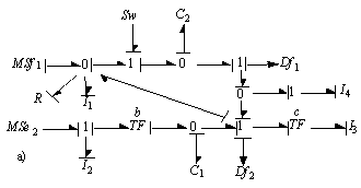Figure 3a. Bond graph model in integral causality (mode 1) : :

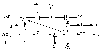Figure 3b. Bond graph model in integral causality (mode 2) : :

There is no storing element in derivative causality in these configurations, so the implicit and explicit state variables are the same and are given by :

.

The application of the derivative causality, for example on mode 1 (Figure 3.a), give the following BGD₁ (Figure 4).

Figure 4. BGD1 + dualization of detectors

We have BG-rank, this mode is observable by continuous outputs Df₁ and Df₂ and discrete output , then the system is structurally observable.

This result can be verified using formal calculation on the bond graph model in integral causality[3].

To study the observability of system (12), it is necessary to apply this result to all modes; if one observable mode exists, the procedure is stopped. The case where no mode is observable, but when the system is observable, can be verified by formal calculation of combined matrix (4).

This calculation can be formally effected :

- by using the bond graph model in integral causality[3], or

- by calculating the observability subspace from bond graph model in derivative causality.

We chose to translate the latter in the form of a second sufficient condition. For that, formal representation of structural observability subspace, denoted as , is given for BG model. It is calculated using causal manipulations. The base of this subspace is used to propose a procedure to study the structural observability of system.

4.2. Graphical Sufficient Condition 2

On the BGD_i (and dualization of continuous and discrete outputs) there exists elements remaining in integral causality and elements in derivative causality.

algebraic equations can be written (Equation (13)) :

(13)

- is either an effort variable for -element in integral causality or a flow variable for -element in integral causality,

- is either an effort variable for -element in derivative causality or a flow variable for - element in derivative causality,

- is the gain of the causal path between the or -elements in integral causality and the or -elements in derivative causality.

Let us consider the column vectors whose components are the coefficients of the variables and in equation (13).

Property 2The column vectors are orthogonal to the structural observability subspace vectors of the mode. We write and .

Procedure 1Calculation of

1) On the BGD_i, dualize the maximum number of output detectors in order to eliminate the elements in integral causality,

2) For each element in integral causality, write the algebraic relations with elements in derivative causality (equation 13),

3) Write a column vector for each algebraic relation with the causal path gains (Equation (13)).

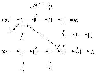Figure 5a. Bond graph model in derivative causality (mode 1)

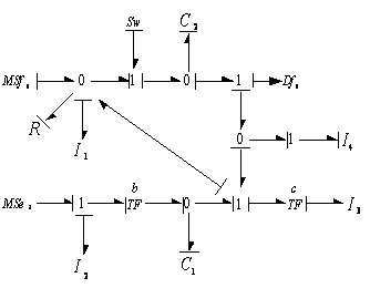Figure 5b. Bond graph model in derivative causality (mode 2)

Example 2 The derivative causality and dualization are now applied to the previous bond graph model where the second detector (Df₂) is removed. The corresponding bond graph models are drawn on Figure 5.

For mode 1, the dynamic element is in integral causality, so wecan write .

The coefficients of the algebraic relation are multiplied by the inductance or capacitance parameter, because of the form of the output matrix in the state equation. Thus we obtain

.

In order to calculate a basis,it is enough to find independent row vectors . These vectors are gathered in the matrix given by

.

In the same manner, from the BGD_i (and dualization of output detectors) algebraic relations can be written (14).

(14)

- is either a flow variable for -element in derivative causality or an effort variable for - element in derivative causality,

- is either a flow variable for -element in integral causality or a flow variable for - element in integral causality,

- is the gain of the causal path between the element in derivative causality and the element in integral causality.

Suppose now the row vectors whose

components are the coefficients of the variables and in equation (14).

Procedure 2 Calculation of

1) On the BGD_i, dualize the maximum number of output detectors in order to eliminate the elements in integral causality.

2) For each element remaining in derivative causality, write the algebraic relation with elements in integral causality, (Equation (14)).

3) Write a row vector for each algebraic relation with the different gains of the causal paths, (Equation (14)).

Property 3The row vectors compose a basis for the structural observability subspace of mode.

With and .

Example 3 We implement procedure 2on the previous example. For mode 1, the two dynamic elements and are not causally connected with , we can write

, the corresponding vectors are

and .

The algebraic equations corresponding to the elements

, and are given by :

,

and 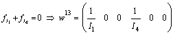. Thus, we have and .

Some calculation is carried out for mode 2. We obtain , with , a, and .

The graphical calculation of structural observability subspaces and remark 2 lead to theorem 5.

Theorem 5 If , the CSLS system is structurally observable.

Proof. We have shown for a given mode that the bond graph model in derivative causality is characterized by an algebraic equation of the form (14) from which, we construct a base of structural observability subspace of the i^th mode, denoted .

After commutation from i^th mode to (i+1)^th mode, implement a derivative causality on the bond graph model and dualization the maximum number of continuous and discrete outputs. We can write another algebraic relation (equation 15).

(15)

Its base is given by .

However, the condition : is sufficient for observability of the system, which implies that condition is also sufficient.

Example 4 Theorem 5 is now applied to the previous bond graph model, we have , then, this system is structurally controllable.

5. Example

Let us consider the following acausal BG model (figure 6).

Figure 6. The acausal BG

This model contains two switches, then we have 4 possible configurations: (mode 1: (Sw₁ closed, Sw₂ closed), mode 2: (Sw₁ closed, Sw₂ open), mode 3: (Sw₁ open, Sw₂ open) and mode 4: (Sw₁ :open, Sw₂ closed)).

■ The bond graph models in integral causality of these modes are shown in figure 7.

Figure 7. The BGIi, a) mode 1, b) mode 2, c) mode 3, d) mode 4

■ Figure 8 presents the bond graphs in derivative causality after dualization of detectors.

Figure 8. BGDi + dualization of detectors

Step 1 : Verification of sufficient condition 1

This step is applied to the 4 modes, but only the mode 1 is presented.

- On the BGI₁, all state variables are in integral causality and are causally connected with the detectors,

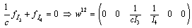
- On the BGD₁, two elements and stays in integral causality. After dualization of the discrete output associated to , only one element remaining in integral causality (figure 8.A), So this mode is not observable.

In the same way, the other modes are not observable, therefore, step 1 is not verified.

Step 2 : Verification of sufficient condition 2

▪ Calculation of W¹ (mode 1)

For mode 1, the element is in integral causality, we have one algebraic relation can be written .

The coefficients of the algebraic relation are multiplied by the inductance or capacitance parameter, because of the form of the output matrix in the state equation. Then .

The algebraic equations corresponding to the elements and are given by: , , then , .

The dynamical element C is not causally connected with , we can write . The corresponding vector is . Thus, we have and .

Same calculation is carried out for the three other modes. We obtain , and , with , , , , , and .

We have

The system is structurally observable.Remark 3 If these conditions are not checked, it is necessary to use a necessary and sufficient condition. This result will be done in a future work.

6. Conclusions

The structural observability property of controlled switching linear systems is studied using simple causal manipulations on the bond graph model. Thus, formal calculation enables us to know the reachable variables; its checking is immediate on the bond graph model in integral causality. On the other hand the bond graph model in derivative causality enables us to characterize graphically the structural observability subspaces relating to each mode. Two sufficient conditionswas given by exploiting these various bases. Finally procedures were proposed.

In fact, the proposed method, based on a bond graph theoretic approach, assumes only the knowledge of the systems structure. The subspaces can be employed to propose structured state feedback matrices in the context of pole assignment by static state feedback. This result can be implemented by classical bond graph theory.

ACKNOWLEDGEMENTS

The author expresses his thanks to the reviewers who made suggestions that helped to improve the presentation of this paper.