Dhouibi H. 1, Nabli L. 1, Hassani M. 1, Craye E. 2
1National school Engineers of Monastir, Road of Kairouan, Monastir, 5000, Tunisia
2Central school of Lille France
Correspondence to: Dhouibi H. , National school Engineers of Monastir, Road of Kairouan, Monastir, 5000, Tunisia.
| Email: |  |
Copyright © 2012 Scientific & Academic Publishing. All Rights Reserved.
Abstract
Quality regulation methodology was developed to control and improve the product and the performance evaluation in Discrete Event Systems (DES). The same particularity may be found on process where the associated constraints do not concern the time. Thus the objective of quality regulation system is to ensure that measure a product’s quality fall into ranges that are acceptable to prospective customers. The control must guarantee the values of the quality variable may or may not fall a random pattern within the limits specified. So a suitable model, rich in analytical properties, is necessary to synthesize the needed controller. The paper is related to the Discrete Events Systems Modelling. We propose a new approach to model the regulation quality systems under temporal and non-temporal constraints. The proposed approach is based on hybrid Petri Nets which combines Interval Constrained Petri Nets (ICPN) and P-temporal Petri Nets. These tools allow us to evaluate the quality variations and to manage the flow type disturbance. The approach is validated on an interesting large scale complex system (more precisely the application is related to a tobacco manufacturing system).
Keywords:
Petri Nets, Regulation, Interval Constraint Petri Nets, Tolerant System, Robust Control
Cite this paper:
Dhouibi H. , Nabli L. , Hassani M. , Craye E. , "A Modelling approach of Robustness Control for Regulation Systems with Temporal and non-Temporal Constraints through Petri Nets", International Journal of Control Science and Engineering, Vol. 2 No. 5, 2012, pp. 93-101. doi: 10.5923/j.control.20120205.01.
1. Introduction
Many practical applications in addition to theoretical developments especially in the area of discrete event dynamic systems were developed. These works were devoted to the design and the synthesis of robust controls for such time constrained processes[1-4]. There was based on the theories and applications of P-temporal Petri Nets systematically[5,6]. These tools are convenient for modelling manufacturing system whose operations times are not precisely given, but are included between a minimum and a maximum value where operations have temporal constraints that must be imperatively respected and the violation of these constraints can damage the health of consumers. The constraint violation causes a deterioration of quality or the stop of production.In many processes, the deciding parameter for the quality and the cost is not time. However, this parameter must strictly belong to some validity intervals. The control must guarantee the fulfilment of these specifications. So a suitable model, rich in analytical properties, is necessary to synthesize the needed controller.The aim of this paper is to explain the use of hybrid PetriNets which combines Interval Constrained Petri Nets (ICPN) and P-temporal Petri Nets. Interval Constrained Petri Nets (ICPN) a sub-class of High Level Petri Nets with Abstract Marking (AM-HLPN)[7,8]. ICPN allow one to model and guarantee a constraint on any parameter of a manufacturing process. P-temporal Petri Nets are convenient tools to model manufacturing systems whose activities times are included between a minimum and a maximum value.Both of tools are applied to a robustness control for regulation systems. We ensure the product quality by verifying density value specifications. The production is optimised by minimizing losses in presence of variation.In the second section the process will be presented.In the third section, we present some usualdefinitions and notations related to the robustness ofmanufacturing systems.Thefourth section describes P-time Petri net and the IntervalsConstrained Petri Nets.In this way, the extension of structural properties of P-Time PN can be justified under some conditions[9].Then we use the production data information to computing methodology was applied in order tobuild the validity intervals of the ICPN model. This tool presents a complement to the P-temporal Petri nets.So we presentthe final model of a robustcontrol laws for manufacturing production systems.Finally, when the ICPN model of the process is completely defined we present an application of the developedapproach to tobacco manufacturing.
2. The Manufacturing Process
One of manufacturing systems where the respect of a produced item’s weight arises is a cigarette making workshop. The process, as shown in (Fig 1), makes a regular and homogenous tobacco pudding (endless cigarette): A beam of tobacco is enveloped by cigarette paper by means of an adhesive. The resulting pudding is cut up into segments corresponding to one cigarette in order to obtain a rough consumed unit (cigarette without filter).Within this process, a weight interval constraint must be respected.In fact, from a quality point of view a too heavy cigarette is difficult to draw and a too light one does not satisfy requirements.The production of cigarettes consists of three steps:-Preparation of a tobacco cut beam that will be setting to obtain a module (m).- Forming of a pudding with density (d) by enveloping the beam with cigarette paper. - Cutting up the pudding into (l) long rough consumed units. Henceforth, such unit is called simply cigarettes.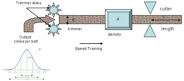 | Figure 1. Steps of a cigarettes making formation in the machine |
A cigarette may be compared to a cylinder with diameter m and length l. Thus, the weight of a cigarette can be expressed by the following relationship: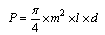 | (1) |
where:m: cigarette’s module in mm with m ∈[mmin, mmax];l:cigarette’s length in mm with l∈[lmin, lmax];d: density in g/mm3 with d ∈[dmin, dmax];
3. Robustness Definitions
Définition1: The robustness of a manufacturing system is defined as its capacityto preserve its specified properties in the presence of expected or unexpected variations. So the robustness of a system characterises its capacity to deal with perturbations.For each system, there are two types of perturbations: internal and external[4]The external robustness of a cell of production is its capacity to conserve the rate of production independently of the fluctuations of its inputs.The internal perturbations are for example variations of operating time, breakdowns of the machine.Definition 2: The passive robustness responds if no modification in control is necessary so that the specified properties are preserved in the presence of variations.Definition 3:The active robustness corresponds if the specified properties can be maintained in case of a total or partial calculation of control.The determination of this robustness provides a decision criterion for the calculation of a new control if the margin of passive robustness is violated (Fig. 2).The Margins A = [a, a’] and B = [b, a [ ] a’, b’] represent the degrees of freedom of the physical process.Each control parameter of a quantitative or qualitative type exceeding these limits involves a violation of the Schedule of Conditions.(1) The specified properties are guaranteed without any change of the control. The values a anda' correspond to the passive robustness.(2) A control must be inventoried; these dynamic margins are modified but the sequencing remains the same. Values b and b’ correspond to the active robustness.
 | Figure 2. margins of robustness |
However the real time computation of a complex system control is not always possible. These considerations lead us to use the robustness proprieties of a part of control architecture in order to decrease the complexity of a synthesis. The aim is to tackle sub-problems which are tractable in real time
4. Petri Nets for the Regulation Control
The exploitation of modeling is adapted as an essential way of research for the determination of the robustness in the production systems. The study of the workshops with temporalor non-temporal constraints contains a singular problem which occurs when one is in the presence of a synchronization mechanism. Since automata do not, by definition, represent inan explicit way the synchronization structures, we choose the Petri nets (P-time Petri Nets andIntervals Constrained Petri Nets) as a modeling tool. In fact, this tool is known as beinga powerful tool ofsynchronization of modeling, parallelisms, conflicts and divisions of resources.The P-time Petri Nets for the study of the workshops with temporal constraintThe theoretical bases of the P-time Petri Nets were elaborated by Khansa in his thesis[10].Hi has shown that they represent a powerful and recognized formalism for modeling the respect obligation of setting times (synchronization under obligation).Definition: P-time Petri Nets is a t-uple ; where
 is a marked Petri net provided with an initial marking and is a definite application per:
 defines the static interval of sitting time of a mark inthe place
  (
( is the set of positive rationalnumbers). A mark in the place
  takes part in the validation of output transitions only if it remained at least the duration in this place. It must leave the place
  at the latest when its setting duration becomes
 . If it cannot do so, we would say that the mark is ’dead’ and won’t take part in the validation of transitions.Interval Constrained Petri NetsICPN are introduced to extend the application[11,12] field of P-Time PN by proceeding to a functional abstraction of the parameter associated places. Naturally, it is logical to find exactly the same mathematical definition of the tool. Nevertheless, if the restriction of the associated parameter to rational numbers is justified when this one is duration, it has no more justification in the case of modelling weight variation or position. Such parameters may take both negative and positive values.Furthermore, the introduction of a new formalism is an opportunity to review the initial definition. Thus, we present in an unequivocal manner the marking as a multi-set. In the same way the transmission of a quantity conveyed by a token is represented explicitly.Definition:An ICPN is a t-uple
 where:•
 is a marked PN•
 is an application associating token to places:Let
  be a set of rational variables.Let
  be a non empty set of formulas to use a variablesof
  . Let
. Let  be a multiset defined on
  .
.
 , where
  is a place marking.We note
  the application:
 (set of positive integer)
 •
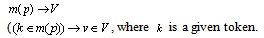
• defines the intervals associated to places. is the set of real numbers.
 •
• is an application that associates to each pair (place, token) a rational variable
  .
.  . Thisvariable corresponds to a modificationof the associated value of a token in a place.
 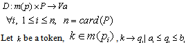 where
where  arerational values fixed by
  •
• is an application that assigns to each variable a value.
 •
• defines the initial values of variables.•
 associates to each token a formula of values in
 is an application of set of the tokens
  in
in  :
: •
• defines to initial formulas associated to tokens.A mark in the place pi is taken into account in transition validations when it has reached a value comprised between ai and bi. When the value is greater than bi the mark is said to be dead. Logically, in the firing of an upstream transition, token are generated in the output places and their associated variable are equal to:
 | (2) |
The signification of q and Val (k) are intentionally not fixed in order to provide a general model.As an example with P-time PN there is the following relation: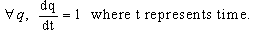 In ICPN the application is not mathematically imposed. We will meet, for example, applications where
  parameters represent weight variations of cigarettes. In this case, parameter values associated to pairs (place, token) are independent. State DefinitionA state
  is defined by a t-uple
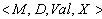 where:
 and
and  are the above defined applications
 and
and  assign a variable
  to each token
  in a place
  A token k of the place
  can take a part in the validation of output transitions if:
  , where [ai, bi] is the static interval associated to the place
 . This token k dies when:
 is an application which provides a value for each variable of
  . Actually, defines the real value of each
  .When
.When  is not defined, there exists a way to make the model evolve. Furthermore, some mathematical properties may be outlined. It is the mathematical abstraction.Definition 2.1: An abstraction on a set {x:A•ψ} may be interpreted as a set a value of the domain associated to the formula A. The A equation using x has to satisfy the constraintψ.The parameters defined with constrained variables will be specified, even though X is not defined, using the above definition:A= Val0(k)+qj,the j index correspond to the visiting order of places by a given tokenx={qj}ψ= (aj≤qi )⊥(qj≤ bi)The analytical conditions of a transition firing will be considered without fixing the final value of q variables. This approach is really useful to make a system specification.Computing the next stepThere are two different ways of reaching a state from a given one. The first solution is to use the evolution of associated variables. The second one is the transition firings. The following two definitions correspond to these two possibilities of evolution.Definition 2.2: A state
  is an accessible from another state
  according to associated variable evolution if and only if:1- m'=m, and2-
  j a token in pi:q’i(j)= qi(j) +Δqi(j),ai≤q’i(j) ≤ biWhere [ai, bi] is the static interval of the place pi.The possibility of reaching q’i(j) depends generally on the coupling with other q evolutions. This particular aspect is not presented hereDefinition 2.3: A state
  is accessible state from another state
  by firing transition tiif and only if:1-ti is validated from E, 2-
 corresponds to the weight of the output arcs from p to ti .
 corresponds to the weight of the input arcs from tito p.3-Tokens that remain in the same place keep the same associated value between E and E'. The newly created tokens take null values for the q counter associated to their new places. The value allocated to the token k’ by Val is:
 where k is a token that is in an input place pj of tiand consumed to fire ti.The previous firing rule allows computing states and accessibility-relationships. The set of the firing sequences from an initial state specifies the PN behaviour as well as sets of accessible markings or validated firing sequences in the case of Autonomous PN.Modelling process with ICPNIt is possible to construct aRdP model of the shop then to study the different laws of order while simulating the statistical distribution of the orders on the diameter.However, it is necessary to assume that the synthesis of the model is subject to mistakes and approximations. In the best of the cases, we could recover on the model the outputs of the shop for various values of the parameters. However, the data corresponding to the real outputs of the shops are available. Then It ispossible to calculate the tolerances of the parameters directly on statistics of the shop. These last results will be logically more correct than those that integrate the imperfections ensuing of the modeling phase;Note that these parameters “(1)” (weight, module, length and density) are related. Obviously, the variation of one of these parameters provides a variation of the weight. When it is outside the validity range, the production has to be rejected or a machine blocking.Our objective is to make sure that the permitted tolerance concerning cigarettes weight will be respected by controlling m, l and d parameters. It must belong to a predefined interval. The aim of the controller is to maintain the weight specification by changing the setting m, l and d parameters, whereas they have to remain in a validity interval.We consider the variations of a parameter are always very small in front of its setting value. So, the above relation may be approximated by the following one doing a first order linearization[13]:
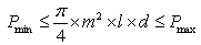 | (3) |
Linearization in the region of a setting pointThe variation of a parameter is always very small in front of its setting value. By the consequence, the above relation may be approximated by the following one doing a first order linearization:ΔP∈[ΔPmin, ΔPmax]Let's consider p0, m0, d0 and l0, respectively the values targets of the parameters p, m, c and l. A linearization of this relation (3) to the neighbourhood of the point of working targets, give the relation simplified following[13]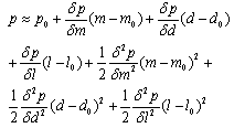 | (4) |
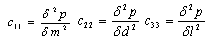
After this development and replacement of increase of this function by the increase in a linear form, the relation (4) becomes: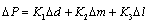 | (5) |
with: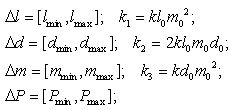 where k is a constant value (∏/4)and p0, m0, d0 and l0, respectively the values targets of the parameters p, m, d and lThese intervals cover margins of active and passive robustness.The equation (5) can be represented by ICPN model shown in fig 3. It called “Weight Value”.Places P1 and P3 are used to limit at one the number of tokens for a specific operation. As they have not other uses we will associate to them the interval (- ∞,+∞ ). They will not restrict, then, the net behaviour.Place P2 models the constraint characterizing module variation.The production process corresponding to places Pd and Pm (density and module) is continuous. It is considered as a discrete one during our study. In fact, module and density measurements are done through pecimens. We consider that twenty cigarettes can give us good representative and reliable information.
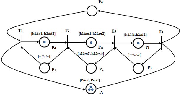 | Figure 3. ICPN model “weight value” |
Density is subject to hazardous variations. Its distribution follows the normal distribution (based on production data). We will then compensate these lapses in acting on the module and length that are adjustable and depend on the state system.However, this regulation should include a coupling system that affects its dynamic behavior.The dynamic behavior of the system is described by the above Petri Net and the validity intervals are well fitted to integrate the validity ranges. However, the problem for now is to compute which value to assign to each interval bound. The next section presents an approach to build them using the statistical production data of the workshop.The industrial problem we propose to tackle with consist in specifying an automatic control using the past production information. This information ensues from a manually non deterministic control. By the consequence there is a great sample of used setting and some of them lead to a workshop blocking and a production waste.When a given setting is often used by a workman, it does not mean that this control is more important than another. The only thing to take into account in this case is the quality of the output. The workman behaviour is not in integrated, because the aim is an automatic control synthesis.The upper limit of diameter is given by the size of the paper used. Each cigarette that falls outside of the user defined range (dead zone), upper or lower can generate a blockage of machine implying a stop of the shop and the loss of all present in - courses in the chain (they are put to the rebus).Mathematically, time PN and any ICPN have the sameproperties. However,the physical interpretation that must be given to the model iscompletely different.Table 1 summarizes significance of different parameters thattake part in both time PN and the ICPN.| Table 1. Comparison of parameters p-time pn/icpnmodel |
| | Parameter | P-timePN signification | ICPN model | | C | Time cycle | Weighting cycle for a piece | | Q | Variation of time cycle | Variation of weight per cycle for a piece (compared to reference) | | ∆Q | Variation of effective time | Variation of the added weight in place compared to a reference | | ai | Lower bound indicates the minimum time neededto execute the operation | Lower bound indicates the minimum weight added otherwisethe quality of product is deteriorated | | bi | The upper bound fixes the maximum time to not exceed | Upper bound indicates the maximum weight added otherwisethe quality of product is deteriorated | | M | Product, resource, constraint | Product, resource, constraint |
|
|
Computing validity intervals of ICPN modelThe relation (4) can be writed:with: 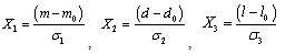 and
and 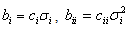 where:
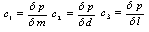
 represents the standard deviation of the considered parameter.The applied data show that the distribution of every quality parameter is symmetrical and follows a normal law. In these conditions and as first approximation we have[14]:
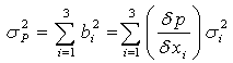 | (7) |
We defined in the previous lines the reasons act on the value of the weight of a cigarette:- Factor 1: the trimmer (module)- Factor 2: The length- Factor 3: The densityFor a traditional experience plan one tries to express the answer (the weight in our case) while making vary the factors. It is possible in the case where one can act on these factors, to make vary them. Then, to given states corresponds an answer.In our case the values of these sizes are uncertain:- The density depends on several parameters as: the practices cultural and certain treatments after harvest. Thesis particularities provide has non deterministic been worth of the density.- The module that is adjustable while acting on the pieces modules of the process (one can decrease or can increase the module but that one cannot fix to an exact value). One can do some measures on samples of cigarettes and can take an average. The fluctuation of the module depends on the state of the pieces of shapes in the process.- The length depends on pieces of cut.To resolve this problem, in this paper we are going to use the statistical data of the shop on the three factors and the answer. And we calculate tolerances thus on these parameters. For it we took the results of measures of these parameters on a production of three months. (usuallywe take the samples of twenty cigarettes all hours).These statistical data of the shop permitted us to determine the standard deviations of the weight, the density and the length that are respectively:σp=20, σd=0.006 σl=and 0.1The application of the relation (7) gives us:such that the values targets for a good quality of cigarettes are: | (8) |
and after simplification the relation (7) gives: | (9) |
Such that the values targets for a good quality of cigarettes are:m0 = 7.94mml0 = 64mmd0= 0.2 g/mm3p0 = 770 mgIn these conditions we can determine the standard deviation of the module while applying the relation (9). σm=0.427.So a tolerance on the module is: ITm = 0.26.The minimum and the maximum tolerances of the parameters are as follows:- Target weight: weight of tobacco rod. It is the target value the system aims to achieve.- Heavy weight: limit relative to the Target weight. Every cigarette heavier than this limit will be ejected.- Light weight: limit relative to the Target weight. Every cigarette heavier than this limit will be ejected. | Figure 4. Validity intervals of the ICPN model |
The figure 4 represents the network ICPN model with the calculated tolerance values.
5. Application: Designs of Experiments
Figure5 describes the global model of the process of Fig 1. To construct this global model with validity intervals, a new modelling tool the Interval Constrained Petri Nets (ICPN) in order to evaluate the variations of the quality of tobacco and P-time Petri Nets to manage the flow type disturbance.  | Figure 5. Global ICPN model with command (flow-quality) |
This model combines both parts of the system: •the continuous part corresponding to the places Pe, Pd and Pl (trimmer, density and length), which presents the tobacco flow. The places P1, P2, P3 present, respectively, the constraints associated to Pe, Pd and Pl. | Figure 6. Regulation weight system |
 | Figure 7. Principe of weight measurement |
•the discrete part corresponding to the places P4, P5 and Ptest, presents the control law. The places present, respectively, the constraints associated to Pe,Pd and test of quality control.In order to respect the length of parallel paths we must have multiple tokens in places Pd and Pp.Thus, when the model is built, it is possible to describe the constraints on the quality parameters which are required for the manufacture of products in accordance with the specifications.This model allows setting the system functioning around a target state.Another policy is to control the workshop whilefollowing the evolution of the parameters in the course of time in order to compensate for the fluctuations.The system described in (Fig. 6) is a rod weight control system for cigarette makers and performs many functions. The trimmer motor (M) consists of an electrodynamics motor whose output shaft is mechanically linked to the trimmer disks through a quadrant gear. By driving the trimmer disks, the tobacco rod weight can be adjusted.This kind of motor allows to carry out rapid and precise movements. Due to a position transducer (T) integrated in the motor, the trimmer disks position is controlled in closed control loop.Data from the scanning unit and are processed in the electronic rack, which sends a correction command to the trimmer if the cigarette is outside of the user definedtolerances.The principle of weight measurement is as follows:The scanning unit provides an electrical signal proportional to the density of the tobacco rod. The electrical signal issued from the scanning unit is converted into binary signal by a 12 bits analog-digital converter. For attributing a weight to binary values provided by the AC-converter, the system applies a transfer function. For a given tobacco and within a restricted range of weight, this transfer function can be approximated by a linear function, i.e. by a line of the form y = ax + b with y milligrams and x bits. In this case ‘a’ and ‘b’ represent the slope and offset of this line.Since a line is given by two measurements (a target and a calibration sample) are sufficient for determining the correct transfer function between real weights and weight determined by the system.The following formula is used for calculating the weight (with given parameters ‘a’ and ‘b’):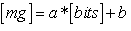 | (10) |
These two parameters are recalculated after each execution of weight correction, standard deviation correction or calibration function but can also be modified manually.Control maintaining constant weightThe effective value of parameter can be calculated with polynomial algorithms. This can be done because the above algorithm is only based upon the structural properties of P-time Petri Net. In this case, it was shown that, under some particular assumptions, the property may be extended to ICPN.A graph G’ is associated with the Strongly Connected P-time Event Graph G in 1-periodic functioning mode of C period:the nodes of G’ are the transitions of G, the arcs of G’ are obtained from the places of G. two arcs are associated with each place p:- the first one from p to p is valued by: | (11) |
-the second one from p to p is valued by: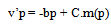 | (12) |
A periodic control of the parameters is obtained with the following algorithm:- choose a transition ts, associate Sts(1) = 0withts- associate with each transition 
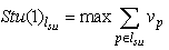 | (13) |
wherelsu is an elementary directed path from s to u. This last algorithm is in O(n3).Computing the robust controlFinally, when the ICPN model of the process is completely defined, it is possible to analyse the structural properties. It was proved that the most of the structural properties of P-time PN can be extended to ICPN[9]. An internal robustness analysis of the ICPN model of the presented process is published in[8].Finally, using the production data information, a computing methodology was applied in order to build the validity intervals of the ICPN model.This approach uses only a sub-part of the information, because we only want to find critical tests which are needed for The Designs of experiments applying in the production data.An observation of the tobacco processing by thedifferent units during one month resulted in picking outthe variations of the output measures: weight, module, depending on the fluctuation of the tobacco density.Fig. 8, Fig 9 andFig 10 represent, respectively, the variation of tobacco weight, density and module.Each figure has plotted control limits that present regulationboundaries, that is, managing boundaries, and a centreline gained by calculating averagearithmetic value of the measurement samples. In our case the measured values are within controllimits, then the process is under controlA centreline (CL),represents the mathematical average of all the samples plotted,UCL and LCL, present respectively, the upper and lower statistical control limits that define the constraints of common causevariations,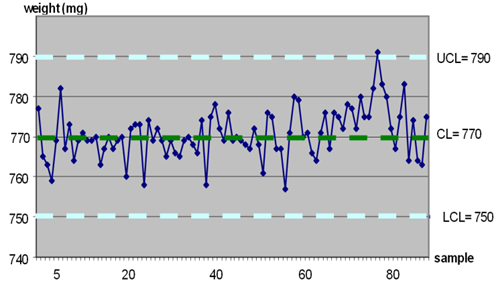 | Figure 8. Variation of weight |
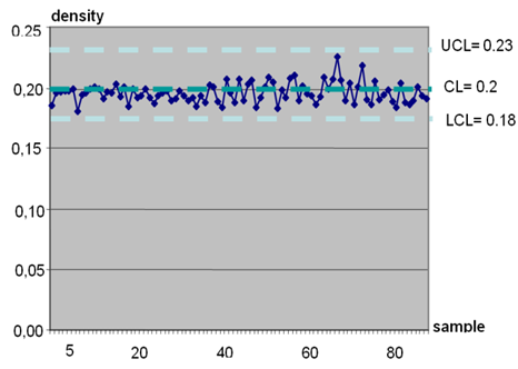 | Figure 9. Variation of density |
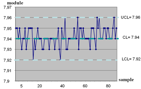 | Figure 10. Variation of module |
6. Conclusions
In this paper, a methodology of design and modeling of control laws is adopted. We modelled by the use of the Intervals Constrained Petri Nets. The ICPN model concerns processes where the conformity of the finished product depends on the value of the weight by a produced unit. This value must belong to a certain validity interval. Outside this interval product is considered as rejection. To improve production performance within such a process, the control of the quality constraint must be able to adjust fluctuations that affect the system’s entries. This adjustment has to be done through intermediate regulations that do not alter specifications. Regulations concern parameters that influence directly the weight. In our case parameters are density (d), module (m) and length (l).ICPN tool which presentsa functional abstraction of the P-temporal Petri Nets; constraintssubjected on flow and quality parameters while integrating themargins of robustness. The goal is to satisfyqualitative and quantitative needs of the market.It is to be noted that the presented data are real production data of an existing workshop. The proposed methodology is therefore validated by a large set of data, and it provides an interesting industrial efficiency for the considered case study.Moreover, theICPN properties may be used for supervision anddiagnosis specifications. Nevertheless thisapplication area still needs to be developed.
ACKNOWLEDGEMENTS
The authors would like to thank the editor and refereesfor their insightful comments that greatly improved thecontentof this paper.
References
| [1] | [JER04] N. Jerbi, S. CollartDutilleul, E. Craye et M. Benrejeb, "Robust Control of Multiproduct Job-shops in Repetitive Functioning Mode", IEEE Conference on Systems, Man, and Cybernetics (SMC’04), The Hague, Vol. 5, pp. 4917–4922, Octobre 2004. |
| [2] | Nabli L., Telmoudi A.J., M’hiri R. (2008), Modeling and analysis of a robust control of manufacturing systems: flow-quality approach, International Journal of Computer, Information, and Systems Science,©www.waset.org, winter. |
| [3] | CollartDutilleul , N. Jerbi,, E. Craye et M. Benrejeb, Robust Control of Multiproduct Job-shops in Repetitive Functioning Mode”, proceeding of MCPL`07, Sibiu, Roumanie, septembre 2007. |
| [4] | CollartDutilleul S., Denat J-P, Chetouane F. « External Robust Control of Eletroplating Line » Conference on Systems, Man, and Cybernetics (SMC’02), Hamamet, Tunisie, 2002. |
| [5] | [CAL97] S. Calvez, P. Aygalinc, and W. Khansa, "P-time PN for manufacturing systems with staying times constraints", IFAC CIS Congress, Belfort, pp. 495–500, Mai 1997. |
| [6] | W. Khansa, J.P. Denat, S. Collart-Dutilleul (1996), "P-Time Petri Nets for Manufacturing Systems". Wodes.96, Edinburgh UK, August 19-21, pp. 94-102, International Workshop on Discret Event System W. Lucky, “Automatic equalization for digital communication,” Bell Syst. Tech. J., vol. 44, no. 4, pp. 547–588, Apr. 1965. |
| [7] | P. Yim, A. Lefort, and Hebrard (1996) "System Modelling with Hypernets" ETFA’96 IEEE Conferences, pp 37-47, Paris.publication),” IEEE J. Quantum Electron., submitted for publication. |
| [8] | CollartDutilleul S., H. Dhouibi and E.Craye. (2003), "Internal RobustnessofDiscret Event System with interval constraints in repetitive functioning mode", ACS'2003 conference, Miedzyzdroje Poland, pp. 353-361. |
| [9] | CollartDutilleul S.,H. Dhouibi and E.Craye (2004)," Tolerance analysis approach with interval constrainted Petri nets", ESMc conference, Paris, pp. 265-272.” |
| [10] | [KHA97] W. Khansa, "Réseaux de Petri P-temporels: Contribution à l’étude des systèmes à événements discrets", Thèse de Doctorat, Université de Savoie, Annecy, mars 1997. |
| [11] | Nabli L., Dhouibi H., Using Interval Constrained Petri Nets for Regulation of Quality: The Case of Weight in Tobacco Factory, International Journal of Intelligent Control and Systems, IJICS, VOL. 13, NO. 3, pp. 178-188, September 2008. |
| [12] | Dhouibi H., CollartDutilleul S., Nabli L. Craye E. (2008)"UsingInterval Constrained Petri Nets forReactive Control Design", theInternational Journal Manufacturing Systems and Production (IJMSP),volume 9, NOs. 3-4, pp217-228, ISSN (printed): 0793-6648, 2008. |
| [13] | Dhouibi H., S. CollartDutilleul, E. Craye and L. Nabli (2005), "Computing An Introduction to Signal Detection and Estimation. Intervals Constrained Petri Nets: a tobacco manufacturing application", IMACS conference, Paris, pp. 440-446. |
| [14] | Maurice Pillet(2000), "Appliquer la Maîtrise Statistique deProcédé",Edition d’Organisation 1995-2000. Pages 395-398. |
 Abstract
 Reference
 Full-Text PDF
 Full-Text HTML