-
Paper Information
- Next Paper
- Previous Paper
- Paper Submission
-
Journal Information
- About This Journal
- Editorial Board
- Current Issue
- Archive
- Author Guidelines
- Contact Us
International Journal of Control Science and Engineering
2012; 2(4): 75-82
doi: 10.5923/j.control.20120204.04
Maximum Allowable Delay Bound Estimation in Networked Control of Bounded Nonlinear Systems
 Abstract
 Reference
 Full-Text PDF
 Full-Text HTML
Ashraf F. Khalil 1, Jihong Wang 2
1School of Electrical, Electronic and Computer Engineering, University of Birmingham, Birmingham, B15 2TT, UK
2School of Engineering, University of Warwick, Coventry, CV4 7AL, UK
Correspondence to: Ashraf F. Khalil , School of Electrical, Electronic and Computer Engineering, University of Birmingham, Birmingham, B15 2TT, UK.
| Email: |  |
Copyright © 2012 Scientific & Academic Publishing. All Rights Reserved.
Networked Control Systems (NCSs) has been recognized as an area where theory is behind the development of technology. The defining feature of NCSs can be considered as the information is exchanged through a network among control system components. So the network induced time delay is inevitable in NCSs. The time delay may degrade the performance of control systems and even destabilize the systems if they are designed without considering the effects of the time delays properly. Once the structure of a NCS is confirmed, it is essential to identify what the maximum time delay is allowed for maintaining the system stability which, in turn, is also associated with the process of controller design. This paper proposes a new method for estimating the maximum allowable time delay in networked control systems with norm bounded nonlinearity. The relation between the maximum nonlinearity and the maximum allowable delay is studied using the proposed method, and it is found that increasing the maximum nonlinearity bound reduces the maximum allowable delay. Furthermore, increasing the time delay leads to shrink the domain of attraction. The results of the maximum allowable delay bound and the maximum nonlinearity are compared with some of the published results.
Keywords: Networked Control System, Stability, Nonlinearity, Norm Bounded, Maximum Allowable Delay Bound
Article Outline
1. Introduction
- The advances in communication and network technology, and the availability of high-speed computers have resulted in an increasing interest in Networked Control Systems (NCSs). This type of control systems can be defined as a control system where the control loop is closed through a real-time communication network[1]. The term “Networked Control Systems” first appeared in Gregory C. Walsh's article in 1998[2]. A typical organization of an NCS is shown in Figure 1. In Networked Control Systems, the reference input, plant output and control input areexchanged through a real-time communication network. The main advantages of NCSs are modularity, simplified wiring, low cost, reduced weight, decentralization of control, integrated diagnosis, simple installation, quick and easy formaintenance[3], flexible expandability (easy to add/remove sensors, actuators or controllers with low cost). NCSs are able to easily fuse global information to make intelligent decisions over large physical spaces.As the control loop is closed through a communication network, the time delay and data dropout are unavoidable. This may degrade the performance of NCSs or even destabilize the system.
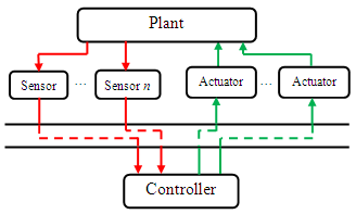 | Figure 1. A Typical Networked System |
2. Mathematical Analysis
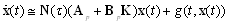
- A nonlinear system is given by:
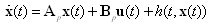 | (1) |
 is the system state vector and
  is the system control input.
  and
and  are matrices with appropriate sizes.
  is the nonlinearity.The nonlinearity is assumed to be piecewise-continuous function of both t and x.
  is uncertain and satisfies the quadratic inequality[14][15];
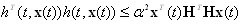 | (2) |
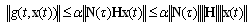
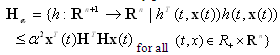 The constraint (2) can be interpreted as[18];
 | (3) |
 | (4) |
 | (5) |
 | (6) |
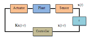 | Figure 2. An NCS with time delay between the sensor and the controller. |
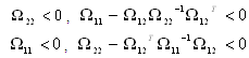
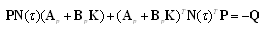
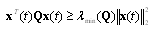
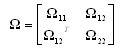 where Ω11, Ω12 and Ω22 are block matrices, and Ω11 is a square matrix. The following three conditions are equal in value:
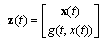
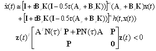
 .Applying (4) into (1);
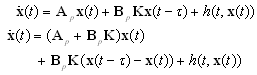 | (7) |
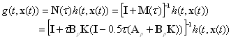
 can be obtained by Taylor Expansion as:
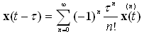 | (8) |
 | (9) |
 | (10) |
 | (11) |
 | (12) |
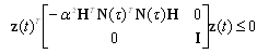
 According to (2) with the time delay the quadratic inequality can be written as;
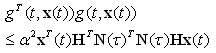 | (13) |
 | (14) |
 | (15) |
 .Choosing the quadratic Lyapunov functional candidate and taking its derivative;
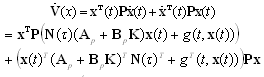
 | (16) |
 | (17) |
 .Following the approach in[18] by combining (15) and (17) we get;
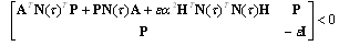 Letting
 and using Lemma 1 we finally get;
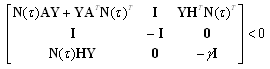 | (18) |
 Theorem 1System (1) and the controller (4) with a given time delay is robustly stable with degree α if the following is feasibleMinimize
  Subject to Y > 0 and (18)The optimization problem in Theorem 1 is quasi-convex optimization in
  which can be solved easily using the Matlab LMI Toolbox. For systems with small time delays where the first derivative approximation can be used, the matrix
  can be approximated as
  , which can lead to less conservative results.Corollary 1Let H.1 holds, then the nonlinear system (1) with the controller (4) is robustly stable with degree α if
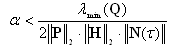 ProofChoosing a Lyapunov functional candidate as:
 | (19) |
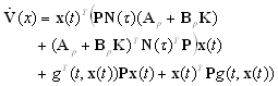
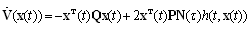
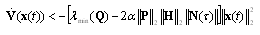
 [19][20]. Taking the derivative of (19) along with the system trajectory (12),
 | (20) |
 | (21) |
 | (22) |
 , there exist
  such that
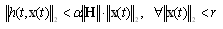 Then;
Then;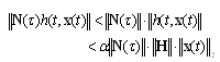 | (23) |
 | (24) |
 | (25) |
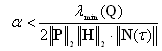 then
then  , the system will be robustly stable with degree
  . We can see from Corollary 1 that the MADB decreases with increasing
  . Setting
  and neglecting the second order term then Corollary 1 reduces to Corollary 1 in[22] as follows;
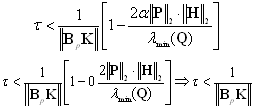 Increasing
  means moving away from the equilibrium point. We noticed as we move away from the equilibrium point the MADB decreases. The boundary of the domain of attraction is when:
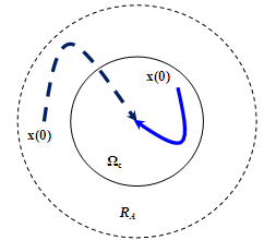
 which means the MADB on the boundary is approximately zero.In NCS with nonlinearity it is important to find or estimate the domain of attraction. The domain of attraction is defined as the region where the limit of every trajectory of the nonlinear system originating in RA is the equilibrium point. RA is shown in Figure 3. It is assumed that the origin is asymptotically stable.In[21] the domain of attraction of the equilibrium point (the origin) is defined as:
 where
where  is the initial state at t = 0. It is difficult to find the domain of attraction but we can estimate a region Ωc, that is ΩcRA, using Lyapunov’s method. The estimate of the domain of attraction Ωc in[21] is defined as:
 | (26) |
 | (27) |
 | (28) |
 | (29) |
 | Figure 3. The region of attraction. |
3. Stability Analysis Case Studies
- In general, two approaches are applied to controller design for NCSs. The first design approach is to estimate the maximum allowable delay bound for the system and then the network is scheduled to limit the time delay to be less than the MADB. The second approach is to design the controller while taking the time delay and data dropouts into account. In this paper, the first approach has been adopted. In this section, a number of examples are studied to demonstrate the approach proposed and compare it with the previously published cases. In particular, the results derived using the method proposed in this paper has been compared with the results using the LMI method given in[14][15]. Example 1The first example has been studied in[14][15] with the sampled-data approach, the system is given by
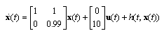 with
with  . The controller is chosen in[14][15] to be
 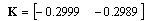 . With
  using Theorem 1 the MADB is 0.292 s. For a time delay,
  s, and using Theorem 1 we have:
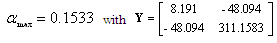 .Using Corollary 1:
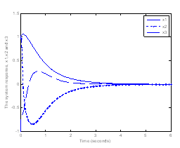
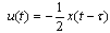
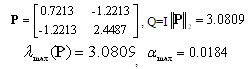 .The maximum nonlinearity bound given in[14][15] is 0.0013. In[24] αmax=0.1636 with 0.2509 s time delay. However Corollary 1 and Theorem 1 still give conservative results the method is very easy compared with the method in[14],[15] and[24]. It is clear that the results of Theorem 1 are less conservative than the results of Corollary 1.The trajectory of the system is shown in Figure 4. For comparison the nonlinear function and the initial conditions for the simulation are given by;
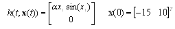 .
.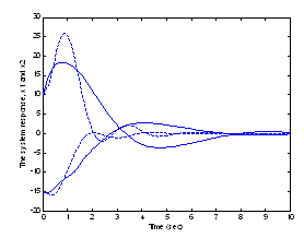 | Figure 4. The system response with zero time delay (solid-line) and 0.2509 s time delay (dashed-line) |
 , the maximum nonlinear bound is αmax=0.1365, using Corollary 1 αmax=0.0256 while using Theorem 1 αmax=0.2555. Here Theorem 1 gives less conservative results than the published ones. The MADB as a function of the nonlinearity is given in Figure 5. It can be easily seen that as the nonlinearity increases the MADB decreases.
 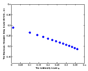 | Figure 5. The MADB as a function of the nonlinearity bound using Theorem 1 |
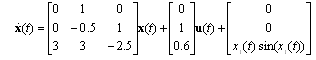 The controller in[17] is designed to be
 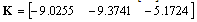 . Setting
  and using theorem 1 the MADB is 0.0601 s. The maximum nonlinearity bound for the delay free system is 4.3. The MADB as a function of the nonlinearity is shown in Figure 6. The system response with 0.03 s and 3 nonlinearity is shown in Figure 7.
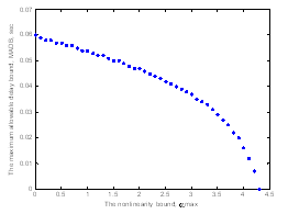 | Figure 6. The MADB as a function of the maximum nonlinearity bound using Theorem 1 |
 | Figure 7. The system response with 0.03 s time delay and α=3 |
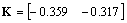
 In[10] the authors use Razumikhin and Lyapunov theorem and the MADB reported in[10] is 2 s. Using Theorem 1 with
 , the MADB is 2 s. Choosing
  ; from (21) we have;
 Choosing
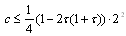
  ;
; .For to be positive
  , so the MADB is 0.366 s. Using Theorem 1 with
  , the MADB is 0.366 s.Using the finite difference approximation for the delay term, the time delay nonlinear system is given by;
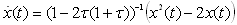 .The system is stable if
  . Choosing Lyapunov functional candidate as;
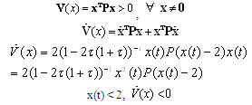 The equilibrium points of the system are:
  and
and  , we will study the domain of the attraction at the origin; for the system to be stable we must have;
  that implies
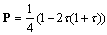
  .The domain of attraction is estimated through using (28);
  where
where 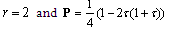 ,
, that implies
  .We can see that increasing the time delay decreases the domain of attraction and when the time delay approaches the MADB then the domain of attraction becomes very small. The system response with different time delays is shown in Figure 8. From Figure 8, the system is still stable even with 0.75 s, which shows that the results of Theorem 1 are still conservative. Figure 9 and Figure 10 show the system response with 0.76 s time delay and 0.15 and 0.5 initial condition respectively.
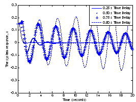 | Figure 8. The system response with different time delays and 0.15 initial condition |
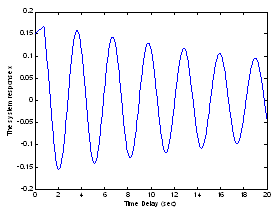 | Figure 9. The system response with 0.76 s time delay and 0.15 initial condition |
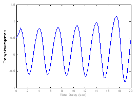 | Figure 10. The system response with 0.76 s time delay and 0.5 initial condition |
4. Conclusions
- The main contribution of the paper is to have derived a new method for estimating the maximum time delay in NCSs with norm bounded nonlinearity. The most attractive feature of the new method is that it is simple in structure and easy for applications, which can be clearly interpreted to design engineers in industrial sectors. The results obtained in this method are compared with those obtained through the methods introduced in other literatures. The method has demonstrated its merits in using less computation time due to its simple structure and giving less conservative results while showing good agreement with other methods. The method is used to estimate the MADB for a given nonlinearity bound which can be used as a guiding tool for the network scheduling. We found that increasing the nonlinearity bound reduces the MADB also increasing the time delay reduces the domain of the attraction for the NCS with bounded nonlinearity.