1. Introduction

The dynamic surface control (DSC) is a dynamic extension of multiple sliding surface (MSS) control to overcome the drawback of "explosion of complexity" in backstepping as well as MSS control[1]. The use of a series of dynamic filters enables the controller to be designed sequentially and simple. Furthermore, the existence of controller gains for semi-global stability was theoretically proved in[1]. Recently, an analysis and design method in the framework of convex optimization has been introduced to allow us to find a quadratic Lyapunov function numerically for a class of nonlinear systems called strict-feedback form[2].

This control approach was extended to a class of nonlinear systems where the uncertainty is linearly parameterized, e.g., in (1) where a is an unknown constant and f₁ is a known nonlinear function. The adaptive backstepping method has been developed[3] and extended to a class of time-delay nonlinear systems[4, 5]. As introduced above, the adaptive DSC to solve the problem of "explosion of complexity" has been developed for a class of nonlinear systems and time-delay systems[6, 7]. Furthermore, DSC has been combined with adaptive neural network control scheme in the literature[8, 9]. However, the useful tools such as linear matrix inequalities (LMIs) are hard to apply to nonlinear system with linearly parameterized uncertainties. There is little work in the literature for LMIs to be used for stability analysis of adaptive nonlinear control problems.

The following example illustrates the design procedure of adaptive dynamic surface control in[6]:

(1)

where a is unknown but bounded by a known positive constant c such that and is a known nonlinear function and locally Lipschitz on , i.e.,

Where y is a Lipschitz constant. The control objective is where x_1d is a constant with, which is called a set-point control problem.

First, define the first error surface as . After taking its derivative along the trajectories of (1)

,the synthetic input, which is to drive, is

(2)

where K is a controller gain and is the estimate of the unknown parameter a following the update law as propose in[6]:

(3)

Where pis a positive constant.

Then, define the second sliding surface as where x_2d equals passed through a first-order filter, i.e.,

(4)

where τ is a filter time constant. Similarly, the derivative of S₂ along the trajectories of (1) is

,and the control input is derive as

(5)

where is calculated from (4) such that

.

It is interesting to remark that the calculation of becomes simpler due to the inclusion of the first-order filter while it results in "explosion of complexity" in backstepping.

A next question is how to design a set of controller gains to guarantee stability, e.g., K, τ and ρ in the example. It was proven in[6] that there exist a set of controller gains (K and τ) to guarantee the stability for stabilization and set-point control problems. However, the performance of the adaptive DSC depends on ρ critically[10]. If a small magnitude of ρ is chosen, the adaption of a in (3) will be slow and the transient error will be large. On the other hand, too large magnitude of ρ will lead to oscillatory estimation of the parameter, thus resulting in the oscillatory error.

Suppose a = 1 in (1), K = 2.5 in (2) and (5), and τ = 0.05 in (4). When ρ is assigned as 1 and 10 respectively, the time responses of x₁ and are shown is Fig. 1. As explained above, the larger magnitude of ρresults in faster convergence of estimation error of and tracking error. However, when ρ = 70, the oscillatory estimation of the parameter is shown in Fig. 1. Thus, the tracking error does not converge to zero. Furthermore, if x_1d is changed to a different constant, although it will be discussed later in Section 4, the different time response (e.g., oscillatory estimation) of may be shown for the same set of K, τ, and ρ.

Figure 1. Time response of x1 and estimate of a with respect to ρ

Motivated by this example, it is unclear what values of ρ and x_1d guarantee stability and convergence of the parameter estimation error for the given set of a controller gain (K) and a time constant (τ). The main contribution of this paper is to derive the augmented closed-loop error dynamics including parameter estimation errors and filter errors in linear differential inclusion form, and to derive the sufficient condition for stability and parameter convergence. Furthermore, the sufficient condition allows us to check stability of the closed-loop system and convergence of estimated parameters by solving the LMI numerically.

Through this paper, we will use the following notation:

is a zero vector and is a zero matrix with appropriate dimensions. is a square identity matrix and is an identity matrix in the sense that all diagonal elements are one whatever the dimension of the matrix is. If is a vector, diag(x) is a diagonal matrix with the vector x forming the diagonal and diag(x,i) (or diag(x,-i)) is a square matrix of size (n+i) with the vector x forming the i th super-diagonal (or sub-diagonal) stands for a positive definite (or semidefinite) matrix, Tr(X) is the sum of all diagonal entries in X.

2. Problem Statement

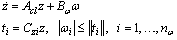
Consider the class of nonlinear system as follows:

(6)

where a_i is an unknown parameter but bounded by a known positive constant c_i such that, f_i and are continuous on and on is a known nonlinear function in strict-feedback form in the sense that the f_i depend only on . It is implied that f_i is locally Lipschitz and is bounded on D_i[11]. Therefore, there exists a constant such that

(7)

for all x on D_i.

3. Adaptive Dynamic Surface Control

3.1. Design Procedure

An outline of the standard design procedure for the adaptive DSC described in[6, 12] is as follows: Define the i th error surface as for where x_1d is the constant value. After taking the time derivative of S_i along the trajectories of (6),

The surface error S_i will converge to zero if , however there is no direct control over the surface dynamics. If x_i+1 is considered as the forcing term for the error surface dynamics, then the sliding condition outside some boundary layer is satisfied if where

(8)

and the update law for the parameter estimate is as follows:

(9)

where K_i is a controller gain and _i is a positive gain.

The next step is to force , so define where equals passed through a first-order filter,

(10)

After continuing this procedure for , define

. After taking its derivative, the control input is

(11)

where is calculated from (10) and the update law of is following

.

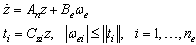
3.2. Augmented Error Dynamics

The augmented closed loop error dynamics is derived for analysis of stability and parameter convergence. After subtracting and adding and , and using u in (11), the closed-loop dynamics in (6) can be written as

for . Using (8) and the definition of error surfaces, the above equations can be described as a function of errors as follows:

(12)

where is the filter error and

is the parameter estimation error multiplied by f_i.

In addition, we need to consider the augmented error dynamics due to inclusion of a set of the first order low pass filters and the update law for the estimate. After taking a derivative of for , the filter error dynamics is

(13)

where the last equality comes from (10). By taking a derivative of (8), we can write as

(14)

for . Since the derivative of h_i is written as

(15)

(14) is rewritten as

(16)

the filter error dynamics in (13) is

(17)

for Equation (15) with the update law in (9) is written as

(18)

can be summarized as

(19)

(20)

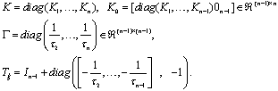
where the vectors are defined asand the submatrices are

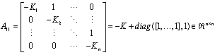
Since the first block matrix in (20) is invertible such that

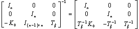where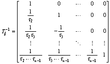

after multiplying the inverse matrix to both sides in (20), the augmented closed-loop error dynamics are written as

(21)

where the error state ,

and the matrices are

where the submatrices are

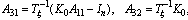
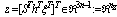
It is noted that the third row of is

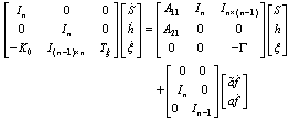
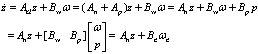
By defining, (21) is rewritten as follows:

(22)

where

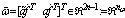
Next, we need to determine the upper bound of ω in (22). Using the assumption in (7), the upper bound of for is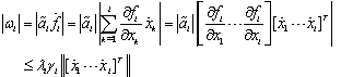

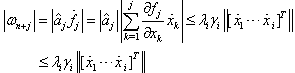for j = 1,…,n-1. Using (12), is written in a function of z as follows:

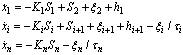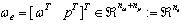
for Therefore, there exists a matrix such that

(23)

Finally, the augmented error dynamics, (19) with the upper bound of ωin (21), can be written in diagonal norm-bounded linear differential inclusion (LDI) form as follows[13]:

(24)

3.3. Quadratic Stability

Since A_cl in (24) is not time invariant due to A₂₁ is (21), both A₂₁ and A₃₁ can be decomposed into a steady-state term and a time varying term under the assumption that as for the given set of controller gains. That is,

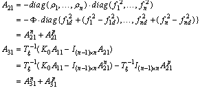where

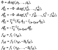and is a nominal constant, e.g., or a rough estimate of a_i. Therefore, A_cl can be written as

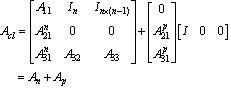(25)

Using (25), (24) can be considered as a nominal closed-loop error dynamics subject to a vanishing perturbation term as follows:

(26)

where

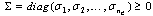
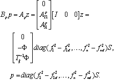Since p is a function of S and is bounded on D, there exists a matrix C_zi such that for i = 2,…,n-1.

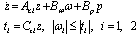
Finally, the augmented error dynamics in (24) can be written as

(27)

Since the augmented error dynamics in (27) is written in diagonal normbounded LDI, its quadratic stability can be applied as follows[13]:

Definition 1. Suppose A_n in (27) is Hurwitz for the given set of controller gains, , and update law gains, . The augmented error dynamics in (27) is quadratically stable if there exists a positive definite matrix p such that

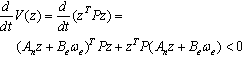(28)

If the error dynamics is quadratically stable, z = 0 is an exponentially stable equilibrium point on D. The sufficient condition above for quadratic stability can be expressed in terms of linear matrix inequality (LMI) as described in the following theorem.

Theorem 1. Suppose that the diagonal norm-bounded error dynamics in (27) is given for given set of controller gains and A_n is Hurwitz. The error dynamics in (27) is quadratically stable on D if there exist P > 0 and such that

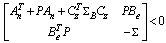(29)

where

,

is the diagonal block matrix.

The equivalence between (28) and (29) can be referred to[13].

Remark 1. If there exists the solution for (29), z = 0 is exponentially stable. That is, x₁→x_1d and as t→∞. Moreover, if f_i satisfies the so called “persistent excitation”[6], i.e., there exist strictly positive constants a_i and T such that for any t > 0,

as t→∞. Otherwise, it is not guaranteed for the estimated parameter to converge to the correct value although x₁→x_1d as t→∞.

4. Illustrative Example

Consider (1) again with the unknown parameter a = 1 and the control objective is x₁→x_1d = 1. Suppose the domain and where c = 2. Then,

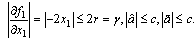If the controller derived in Section 1 is applied, the closed-loop error dynamics is following as in (19):

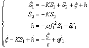(30)

where and . Equation (30) can be written in matrix form as follows:

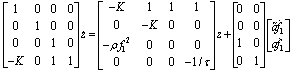(31)

where . As derived in (22), (31) can be writtens as

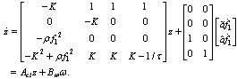where and the upper bound of w is determined as follows:

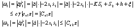where and

Therefore, the augmented error dynamics can be written in LDI form as

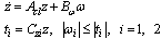(32)

For stability analysis, (32) is considered as a perturbed system as follows:

(33)

where the matrices are

is a vanishing perturbation and its upper bound is

where m is a maximum of f₁ on D, i.e., ,

and .

Finally, the augmented error dynamics is written in diagonal norm-bouned LDI as

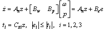(34)

The eigenvalues of A_n in (34) are caculated as following:

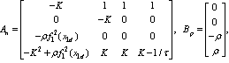
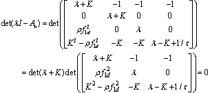where . Then,

It is noted that the decond characteristic equation can be derived using Symbolic Math Toolbox of MATLAB. Using the Routh stability criterion, the inequality condition for A_n to be Hurwitz is derived to be

(35)

Suppose K = 2.5 and τ = 0.05. Then, the inequality condition in (35) becomes

If three values of ρare considered, i.e., ρ_i={1,10,70}, i = 1,2,3, three ranges of x_1d for A_n to be Hurwitz are obtained as follows:

(36)

That is, for ρ₁ = 1, for ρ₂ = 10 and for ρ₃ = 70.

When x_1d = 1 and ρ_i is either 1 or 10, the matrix A_n in (32) is Hurwitz for both cases and LMI (29) can be solved via convex optimethod called CVX[14] is used to solve the feasibility problem by calculating P and Σ in (29) numerically in the framework of MATLAB. As predicted through stability analysis, x₁→x_1d and as t→∞ as shown in Fig. 1. For ρ₃ = 70, the eigenvalues of A_n are

Since the matrix A_n is not Hurwitz, this results in the oscillatory estimate of a and thus oscillatory tracking of (refer to Fig 1).

If x_1d is changed to 1.5, the eigenvalues of A_n with respect to ρ_i are

for,

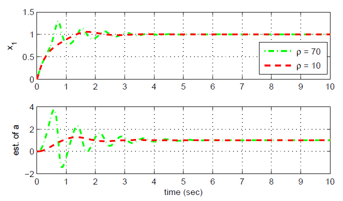
for.It is shown in Fig. 2 that the time responses of for x₁ and are oscillatory for ρ₂ while the tracking error and parameter estimation error converges to zero for ρ₁. If τ becomes smaller as 0.01, the inequality condition in (36) is modified as

(37)

Thus, the matrix A_n is Hurwitz for all ρ_i and there exist a solution for LMI (29). The corresponding time responses of x₁ and are shown in Fig. 3. It is remarked that a smaller gain of τ allows us to enlarge the range of x_1d for A_n to be Hurwitz. However, it is well known that 1/τ in the first-order filter is a cut-off frequency and the noise thus may not be attenuated if τ is too small.

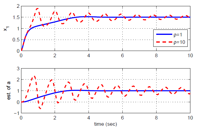Figure 2. Time response of x1 and with respect to ρfor x1d =1.5

Figure 3. Time response of x1 and with respect to ρfor

5. Conclusions

The analysis method for stability and parameter convergence of adaptive dynamic surface control was proposed by deriving the augmented closed-loop error dynamics in linear differential inclusion form. The sufficient condition for stability is derived for the given controller gains in the form of linear matrix inequality. It allows us to analyze both quadratic stability and parameter convergence by computing a quadratic Lyapunov function numerically via convex optimization.

ACKNOWLEDGEMENTS

This research was supported by the Industrial Strategic Technology Development Program (10035250, Development of Spatial Awareness and Autonomous Driving Technology for Automatic Valet Parking) funded by the Ministry of Knowledge Economy (MKE, Korea).