Petr Dolezel1, Libor Havlicek1, Jan Mares2
1Faculty of Electrical Engineering and Informatics, University of Pardubice, 532 10 Pardubice, Czech Republic
2Department of Computing and Control Engineering, Institute of Chemical Technology, 166 28 Prague, Czech Republic
Correspondence to: Petr Dolezel, Faculty of Electrical Engineering and Informatics, University of Pardubice, 532 10 Pardubice, Czech Republic.
| Email: |  |
Copyright © 2012 Scientific & Academic Publishing. All Rights Reserved.
Abstract
The contribution is focused on helicopter elevation control. The experiments are performed on helicopter model, which is significantly nonlinear plant and it simulates in some simplified way dynamics of real helicopter. There is derived new way to control it which uses piecewise-linear neural model. As it is shown at the end of the paper, this new control algorithm brings decent performance improvement compared to certain classical control technique.
Keywords:
Artificial Neural Network, Nonlinear Process Control, Helicopter Model, Piecewise-Linear Model
1. Introduction
Artificial Neural Network (ANN) is a popular methodology nowadays with lots of practical and industrial applications. As introduction it is necessary to mention applications as mathematical modelling of bioprocesses in[1],[2], prediction models and control of boilers, furnaces and turbines in[3] or industrial ANN control of calcinations procedures and iron ore processes[4].Therefore, the aim of the contribution is to explain how to use ANN with piecewise-linear activation functions in hidden layer in control of significantly nonlinear plant (helicopter model). To be more specific, there is described technique of controlled plant linearization using ANN nonlinear model. Obtained linearized model is in a shape of linear difference equation.
2. Helicopter Model
Helicopter model is twin rotor aerodynamic system (Figure 1, Figure 2 and Figure 3) which is designed to simulate real copter dynamics. As controlled plant, it is significantly nonlinear system with two inputs (power of main rotor u and power of tail rotor) and two outputs (vertical elevation yS and yaw motion). All quantities are pronounced as unified voltage signals 0-5V. The aim of this contribution is vertical elevation control, so yaw motion is locked. It is shown further, that classical control techniques (e.g. PID control) do not afford suitable control performances. 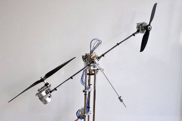 | Figure 1. Helicopter model |
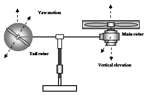 | Figure 2. Helicopter model formal scheme |
In Figure 4, it is shown the response of the plant to defined sum of step functions as example of highly nonlinear dynamics of the plant.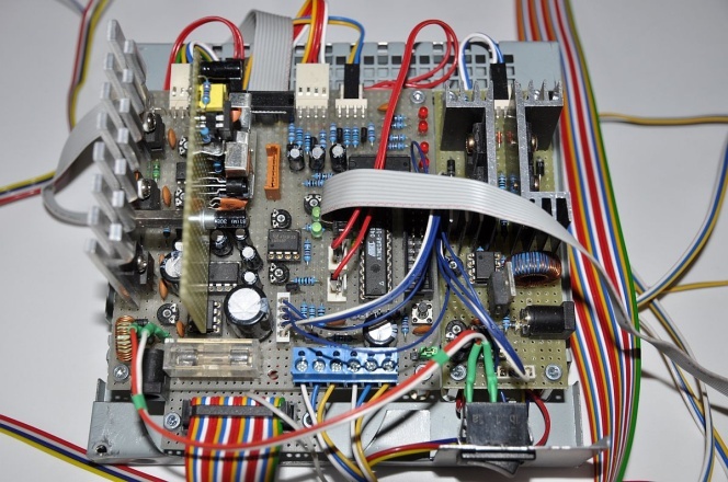 | Figure 3. Control unit of helicopter model |
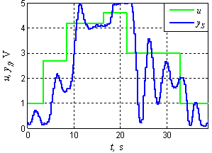 | Figure 4. Response to sum of step functions |
3. Artificial Neural Network for Approximation
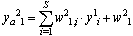
According to Kolmogorov's Superposition Theorem, any real continuous multidimensional function can be evaluated by sum of real continuous one-dimensional functions, see[5]. If the theorem is applied to ANN, it can be said that any real continuous multidimensional function can be approximated by certain three-layered ANN with arbitrary precision. Topology of that ANN is depictured in Figure 5. Input layer brings external inputs x1, x2, …, xP into ANN. Hidden layer contains S neurons, which process sums of weighted inputs using continuous, bounded and monotonic activation function. Output layer contains one neuron, which processes sum of weighted outputs from hidden neurons. Its activation function has to be continuous and monotonic.So ANN in Figure 5 takes P inputs, those inputs are processed by S neurons in hidden layer and then by one output neuron. Dataflow between input i and hidden neuron j is gained by weight w1j,i. Dataflow between hidden neuron k and output neuron is gained by weight w21,k. Output of the network can be expressed by following equations.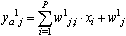 | (1) |
 | (2) |
 | (3) |
 | (4) |
In equations above, φ1(.) means activation functions of hidden neurons and φ2(.) means output neuron activation function.As it is mentioned above, there are some conditions applicable for activation functions. To satisfy them, there is used mostly hyperbolic tangent activation function (eq. 5) for neurons in hidden layer and identical activation function (eq. 6) for output neuron. | (5) |
 | (6) |
Mentioned theorem does not define how to set number of hidden neurons or how to tune weights. However, there have been published many papers which are focused especially on gradient training methods (Back-Propagation Gradient Descend Alg.) or derived methods (Levenberg-Marquardt Alg.) – see[6].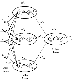 | Figure 5. Three-layered ANN |
4. System Identification by Artificial Neural Network
System identification means especially a procedure which leads to dynamic model of the system. ANN has traditionally enjoyed considerable attention in system identification because of its outstanding approximation qualities. There are several ways to use ANN for system identification. One of them assumes that the system to be identified (with input u and output yS) is determined by the following nonlinear discrete-time difference equation.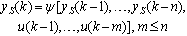 | (7) |
In equation above, ψ(.) is nonlinear function, k is discrete time and n is difference equation order.The aim of the identification is to design ANN which approximates nonlinear function ψ(.). Then, neural model can be expressed by (eq. 8).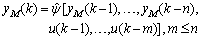 | (8) |
 | Figure 6. Three-layered ANN |
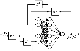
In (eq. 8),  represents well trained ANN and yM is its output. Formal scheme of neural model is shown in Figure 6. It is obvious that ANN in Figure 6 has to be trained to provide yM as close to yS as possible. Existence of such a neural network is guaranteed by Kolmogorov's Superposition Theorem and whole process of neural model design is described in detail in[6].
5. Piecewise-Linear Neural Model
As mentioned in section 3, there is recommended to use hyperbolic tangent activation function for neurons in hidden layer and identical activation function for output neuron in ANN used in neural model. However, if linear saturated activation function (eq. 9) is used instead, ANN features stay similar because of resembling courses of both activation functions (see Figure 7).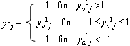 | (9) |
The output of linear saturated activation function is either constant or equal to the input so neural model which uses ANN with linear saturated activation functions in hidden neurons acts as piecewise-linear model. One linear submodel turns to another when any hidden neuron becomes saturated or becomes not saturated.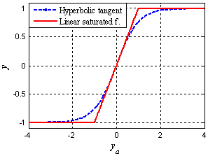 | Figure 7. Activation functions comparison |
Let us presume an existence of some dynamic neural model which uses ANN with linear saturated activation functions in hidden neurons and identic activation function in output neuron – see Figure 6. ANN output can be computed using eqs. (1), (2), (3), (4). However, another way for ANN output computing is useful. Let us define saturation vector z of S elements. This vector indicates saturation states of hidden neurons – see (eq. 10).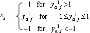 | (10) |
Then, ANN output can be expressed by (eq. 11).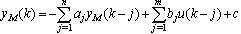 | (11) |
Where: 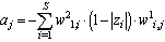 ,
,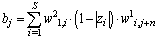 ,
,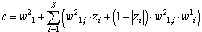 Thus, difference equation (11) defines ANN output and it is linear in some neighbourhood of actual state (in that neighbourhood, where saturation vector z stays constant). Difference equation (11) can be clearly extended into any order.In other words, if it is designed neural model of any nonlinear system in form of Figure 8, then it is simple to determine parameters of linear difference equation which approximates system dynamics in some neighbourhood of actual state. This difference equation can be used then to the actual control action setting due to any of classical or modern control techniques.
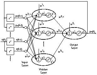 | Figure 8. Piecewise-linear neural model |
If chosen control technique requires model in form of difference equation with no constant term (c = 0), (eq. 11) can be transformed in following way. Let us define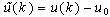 | (12) |
where u0 is constant. Then, (eq. 11) turns into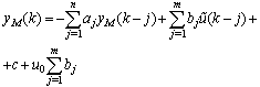 | (13) |
Equation (13) becomes constant term free, if (eq. 14) is satisfied. | (14) |
6. Pole Assignment Technique
Pole Assignment control technique (PA)[7] is polynomial approach to process control which is well usable together with piecewise-linear neural model. The technique forces the whole control loop to some defined behaviour. In other words, it determines controller parameters so that the control loops dynamics is close to defined standard. Suppose the control loop in Z domain as shown in Figure 9.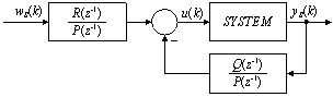 | Figure 9. Pole Assignment Control Technique |
Controlled system should be described by polynomials A(z-1), B(z-1), where polynomial parameters are equal to difference equation parameters used for linear model of the controlled system. Both feedforward and feedback part of controller are defined by polynomials P(z-1), Q(z-1), R(z-1). Z transfer function of closed loop is defined by (eq. 15).While the polynomials A(z-1), B(z-1) are given by the system to be controlled, the other polynomials should be tuned to obtain suitable control response (polynomial R(z-1) affects the closed loop gain and polynomials P(z-1), Q(z-1) are responsible for control performance dynamics).If the system to be controlled is highly nonlinear, the polynomials A(z-1), B(z-1) should be adapted continuously and one simple and suitable way to do it is presented in paragraph 5 – see formal diagram in Figure 10.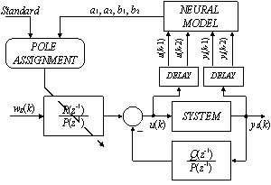 | Figure 10. Pole Assignment with continuous linear model adaptation using piecewise-linear neural model |
7. Helicopter Model Elevation Control
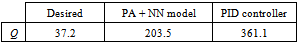
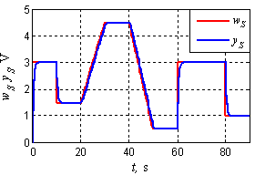
Discrete neural model of the plant (sampling period 0.2s) is designed according to information described in section 4. This procedure involves training and testing set acquisition, neural network training and pruning and neural model validating. As this sequence of processes is illustrated closely in many other publications[6], it is not referred here in detail.Pole Assignment technique is used then for control. Standard for this demonstration is defined as discrete first order system with unit gain – see Z transfer function (16). The aim is to determine continuously (every time instant of control performance) controller polynomials to unify transfer functions (15) and (16), which is simple algebraic task. Control response defined by this standard (desired control response) for some demonstrative setpoint course is shown in Figure 11, while control performance obtained from real device is figured in Figure 12 (yS means real elevation, wS its desired value, t is continuous time). The results are confronted to control performance gained using PID controller tuned by Nichols-Ziegler method[8] (see Figure 13). Control qualities are expressed by quadratic performance criterion (17) – less is better – and numeric values can be found in Table 1.Table 1. Quadratic performance criterion
 |
| |
|
 | Figure 11. Desired control performance defined by (16) |
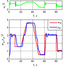 | Figure 12. Control response using PA + Neural model |
8. Conclusions
The paper is focused on the usage of neural network with linear saturated activation functions in helicopter model elevation control. Neural model with such a neural network within is suitable for controller design using any of huge set of classical or modern control techniques. Pole Assignment technique is chosen in this particular case. Control response of real device (Figure 12) should tend to control response defined as standard (Figure 11). However, this is hardly achieved, because highly nonlinear dynamics of the plant cannot be forced to such a smooth course. Nevertheless, comparison to control performance provided by PID controller (Figure 13), which is the most widespread controller in industry, proves decent improvement of control quality.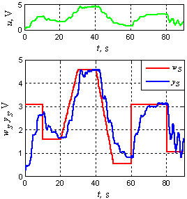 | Figure 13. Control response using PID controller |
ACKNOWLEDGEMENTS
The work has been supported by the funds No. SGFEI03/2012 of the University of Pardubice, Czech Republic. This support is very gratefully acknowledged.
References
| [1] | Gary Montague, Julian Morris, “Neural network contributions in biotechnology”, Elsevier Sci Ltd., Trends in biotechnology, Vol. 12, no 8, pp. 312-324, 1994. |
| [2] | Ana Teixeira, Carlos Alves, Paula Alves, Manuel Carrondo, Rui Oliveira, “Hybrid metabolic flux analysis/artificial neural network modeling of bioprocesses”, in Proceedings of the 5th International Conference on Hybrid Intelligent Systems, pp. 411-416, 2005. |
| [3] | Janusz Lichota, Maciej Grabowski, “Application of artificial neural network to boiler and turbine control”, Kaprint, Rynek Energii, Vol. 16, no. 1, pp. 99-107, 2010. |
| [4] | Srinivas Dwarapudi, P.K. Gupta, Mohan S. Rao, “Prediction of iron ore pellet strength using artificial neural network model”, Iron Steel Inst. Japan, ISIJ International, Vol. 47, no. 1, pp. 67-72, 2007. |
| [5] | Robert Hecht-Nielsen, “Kolmogorovʼs mapping neural network existence theorem”, in Proc 1987 IEEE International Conference on Neural Networks, pp. 11-13, 1987. |
| [6] | Simon Haykin, Neural Networks: A Comprehensive Foundation, Prentice Hall. New Jersey, USA, 1994. |
| [7] | Kenneth J. Hunt, Polynomial methods in optimal control and filtering, Peter Peregrinus Ltd., Stevenage, UK, 1993. |
| [8] | John G. Ziegler, Nathaniel B. Nichols, “Optimum settings for automatic controller” Trans. ASME, vol. 65, no. 1, pp. 433-444, 1942 |
 Abstract
 Reference
 Full-Text PDF
 Full-Text HTML